Causality for Machine Learning
FF13 · ©2020 Cloudera, Inc. All rights reserved
This is an applied research report by Cloudera Fast Forward Labs. We write reports about emerging technologies. Accompanying each report are working prototypes that exhibit the capabilities of the algorithm and offer detailed technical advice on its practical application. Read our full report on causality for machine learning below or download the PDF. Also be sure to check out the complementary prototype, Scene.
Introduction
In recent years, machine learning has made remarkable progress, providing novel capabilities like the creation of sophisticated, computable representations of text and images. These capabilities have enabled new products, such as image searches based on image content, automatic translation between many languages, and even the synthesis of realistic images and voice. Simultaneously, machine learning has seen widespread adoption in the enterprise for classic use cases (for instance, predicting customer churn, loan defaulting, and manufacturing equipment failure).
Where machine learning has been successful, it has been extraordinarily so.
In many cases, that success can be attributed to supervised learning on large volumes of training data (combined with extensive computation). Broadly, supervised learning systems excel at one task: prediction. When the goal is to predict an outcome, and when we have many examples of that outcome arising, as well as the features associated with it, we may turn to supervised learning.
As machine learning has gained popularity, its sphere of influence in business processes has expanded beyond narrow prediction and into decision making. The results of machine learning systems are routinely used to set credit limits, anticipate manufacturing equipment failures, and curate our various news feeds. As individuals and businesses seek to learn from the information provided by such complex and nonlinear systems, more (and better) methods for interpretability have been developed, and this is both healthy and important.
However, there are fundamental limits to reasoning based on prediction alone. For instance, what will happen if a bank increases a customer’s credit limit? Such questions cannot be answered by a correlative model built on previously observed data, because they involve a possible change in the customer’s choices as a reaction to the change in credit limit. In many cases, the outcome of our decision process is an intervention - an action that changes something in the world. As we’ll demonstrate in this report, purely correlative predictive systems are not equipped for reasoning under such interventions, and hence are prone to biases. For data-informed decision making under intervention, we need causality.
Even for purely predictive systems, which is very much the forte of supervised learning, applying some causal thinking brings benefits. Causal relationships are by their definition invariant, meaning they hold true across different circumstances and environments. This is a very desirable property for machine learning systems, where we often predict on data that we have not seen in training; we need these systems to be adaptable and robust.
The intersection of causal inference and machine learning is a rapidly expanding area of research. It is already yielding capabilities that are ready for mainstream adoption - capabilities which can help us build more robust, reliable, and fair machine learning systems.
This report is an introduction to causal reasoning as it pertains to much data science and machine learning work. We introduce causal graphs, with a focus on removing the conceptual barriers to understanding. We then use this understanding to explore recent ideas around invariant prediction, which brings some of the benefits of causal graphs to high dimensional problems. Along with the accompanying prototype, we show how even classic machine learning problems, like image classification, can benefit from the tools of causal inference.
Background: Causal Inference
In this chapter, we discuss the essentials of causal reasoning (particularly in how it differs from supervised learning) and give an informal introduction to structural causal models. Grasping the basic notions of causal modeling allows for a much richer understanding of invariance and generalization, which we discuss in the next chapter, Causality and Invariance.
Why are we interested in causal inference?
Imagine a bank that would like to reduce the number of business loans which default. Historical data and sophisticated supervised learning techniques may be able to accurately identify which loans are likely to default, and interpretability techniques may tell us some features that are correlated with (or predictive of) defaulting. However, to reduce the default rate, we must understand what changes to make, which requires understanding not only which loans default, but why the loans default.
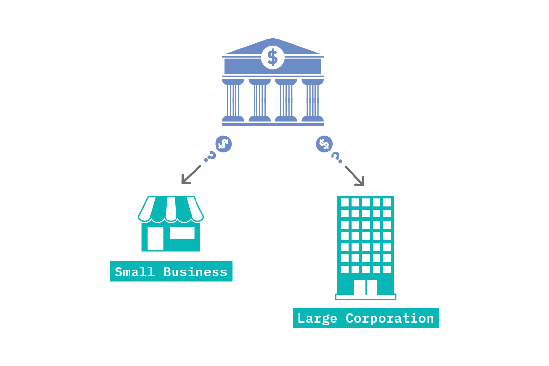
It may be that we find small loans are more likely to default than larger loans. One might naively assume that the bank ought to stop making small loans. However, perhaps it is really the case that smaller businesses are more likely to fail than large businesses, and also more likely to apply for small loans. In this case, the true causal relationship is between the size of the business and defaulting, and not between the size of the loan and defaulting. If this is so, our policy decisions should be influenced by business size, rather than loan size.
Unfortunately, supervised learning alone cannot tell us which is true. If we include both loan size and business size as features in our model, we will simply find that they are both related to loan defaulting, to some extent. While that insight is true - as they are both statistically related to defaulting - which causes defaulting is a separate question, and the one to which we want the answer.
Causality gives us a framework to reason about such questions, and recent developments at the intersection of causality and machine learning are making the discovery of such causal relationships easier.
The shortcomings of supervised learning
Supervised machine learning has proved enormously successful at some tasks. This is particularyly true in dealing with tasks that require high-dimensional inputs, such as computer vision and natural language processing. There has been truly remarkable progress over the past two decades, and it should be noted that an acknowledgment of supervised learning’s shortcomings does not in any way diminish that progress.
With success have come inflated expectations that autonomous systems be capable of independent decision-making, and even human-like intelligence. Current machine learning approaches are unable to meet those expectations, owing to fundamental limitations of pattern recognition.
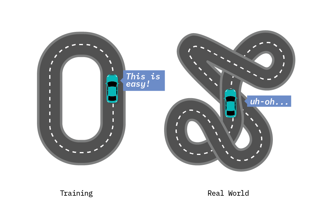
One such limitation is generalizability (also called robustness or adaptability), that is, the ability to apply a model learned in one context in a new environment. Many current state-of-the-art machine learning approaches assume that the trained model will be applied to data that looks the same as the training data. These models are trained on highly specific tasks, like recognizing dogs in images or identifying fraud in banking transactions. In real life, though, the data on which we predict is often different from the data on which we train, even when the task is the same. For example, training data is often subject to some form of selection bias, and simply collecting more of it does not mitigate that.
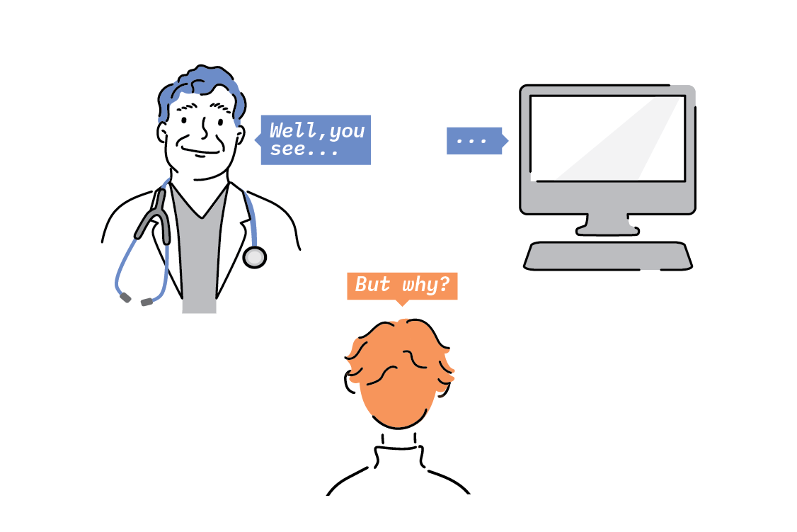
Another limitation is explainability, that is, machine learning models remain mostly “black boxes” that are unable to explain the reasons behind their predictions or recommendations, thus eroding users’ trust and impeding diagnosis and repair. For example, a deep learning system can be trained to recognize cancer in medical images with high accuracy, provided it is given plenty of images and compute power, but - unlike a real doctor - it cannot explain why or how a particular image suggests disease. Several methods for understanding model predictions have been developed, and while these are necessary and welcome, understanding the interpretation and limitations of their outputs is a science in itself. While model interpretation methods like LIME and SHAP are useful, they provide insight only into how the model works, and not into how the world works.
And finally, the understanding of cause-and-effect connections - a key element of human intelligence - is absent from pattern recognition systems. Humans have the ability to answer “what if” kinds of questions. What if I change something? What if I had acted differently? Such interventional, counterfactual, or retrospective questions are the forte of human intelligence. While imbuing machines with this kind of intelligence is still far-fetched, researchers in deep learning are increasingly recognizing the importance of these questions, and using them to inform their research.[1]

All of this means that supervised machine learning systems must be used cautiously in certain situations - and if we want to mitigate these restrictions effectively, causation is key.
What does causality bring to the table?
Causal inference provides us with tools that allow us to answer the question of why something happens. This takes us a step further than traditional statistical or machine learning approaches that are focused on predicting outcomes and concerned with identifying associations.
Causality has long been of interest to humanity on a philosophical level, but it has only been in the latter half of the 20th century (thanks to the work of pioneering methodologists such as Donald Rubin and Judea Pearl), that a mathematical framework for causality has been introduced. In recent years, the boom of machine learning has enhanced the development of causal inference and attracted new researchers to the area.
Identifying causal effects helps us understand a variety of things: for example, user behavior in online systems,[2] effect of social policies, risk factors of diseases. Questions of cause-and-effect are also critical for the design of data-driven applications. For instance, how do algorithmic recommendations affect our purchasing decisions? How do they affect a student’s learning outcome or a doctor’s efficacy? All of these are hard questions and require thinking about the counterfactual: what would have happened in a world with a different system, policy, or intervention? Without causal reasoning, correlation-based methods can lead us astray.
That said, learning causality is a challenging problem. There are broadly two situations in which we could find ourselves: in one case, we are able to actively intervene in the system we are modeling and get experimental data; in the other, we have only observational data.
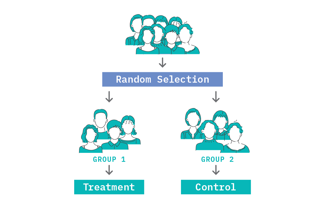
The gold standard in establishing causal effects is a Randomised Controlled Trial (RCT) and this falls under the experimental data category. In an RCT, we try to engineer similar populations using random assignment (as choosing the populations manually could introduce selection effects that destroy our ability to learn causal relations) and apply an intervention to one population and not the other. From this, we measure the causal effect of changing one variable as a simple difference in the quantity of interest between the two populations.
We can use RCTs to establish whether a particular causal relation holds. However, trials are not always physically possible, and even when they are, they are not always ethical (for instance, it would not be ethical to deny a patient a treatment that is reasonably believed to work, or trial a news aggregation algorithm designed to influence a person’s mood without informed consent).[3] In some cases, we can find naturally occurring experiments. In the worst cases, we’re left trying to infer causality from observational data alone.
In general, this is not possible, and we must at least impose some modeling assumptions. There are several formal frameworks for doing so. For our purpose of building intuition, we’ll introduce Judea Pearl’s Structural Causal Model (SCM) framework in this chapter.[4]
The ladder of causation
In The Book of Why, Judea Pearl, an author of much foundational work in causality, describes three kinds of reasoning we can perform as rungs on a ladder. These rungs describe when we need causality, and what it buys us.[5]
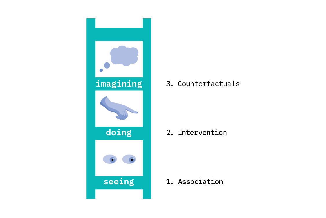
On the first rung, we can do statistical and predictive reasoning. This covers most (but not all) of what we do in machine learning. We may make very sophisticated forecasts, infer latent variables in complex deep generative models, or cluster data according to subtle relations. All of these things sit on rung one.
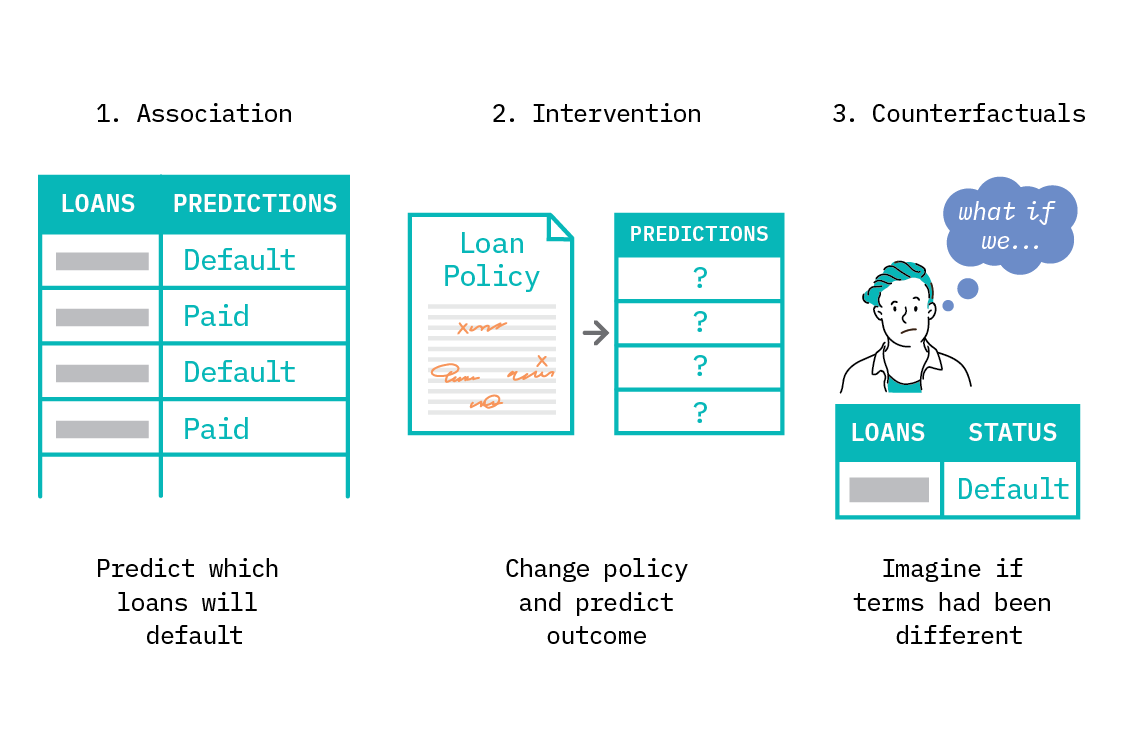
Example: a bank wishes to predict which of its current business loans are likely to default, so it can make financial forecasts that account for likely losses.
The second rung is interventional reasoning. Interventional reasoning allows us to predict what will happen when a system is changed. This enables us to describe what characteristics are particular to the exact observations we’ve made, and what should be invariant across new circumstances. This kind of reasoning requires a causal model. Intervening is a fundamental operation in causality, and we’ll discuss both interventions and causal models in this chapter.
Example: a bank would like to reduce the number of loans which default, and considers changing its policies. Predicting what will happen as a result of this intervention requires that the bank understand the causal relations which affect loan defaulting.
The third rung is counterfactual reasoning. On this rung, we can talk not only about what has happened, but also what would have happened if circumstances were different. Counterfactual reasoning requires a more precisely specified causal model than intervention. This form of reasoning is very powerful, providing a mathematical formulation of computing in alternate worlds where events were different.
Example: a bank would like to know what the likely return on a loan would have been, had they offered different terms than they did.
By now, we hopefully agree that there is something to causality, and it has much to offer. However, we have yet to really define causality. We must begin with a familiar refrain: correlation is not causation.
From correlation to causation
Spurious correlations
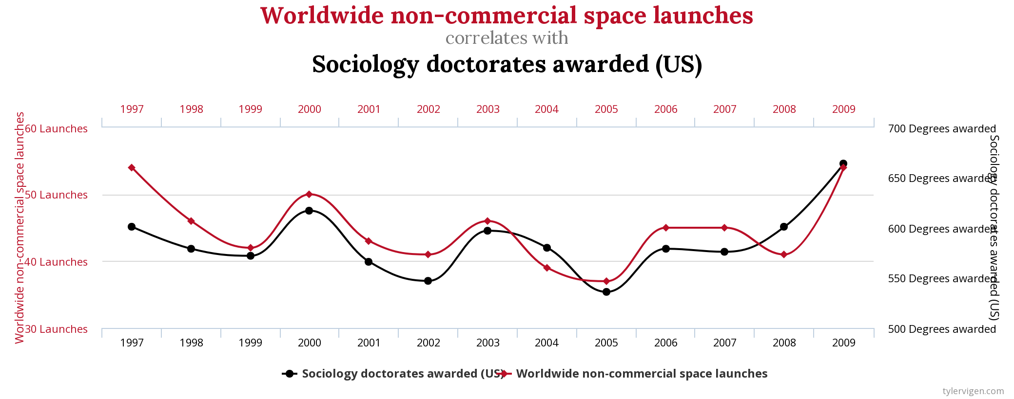
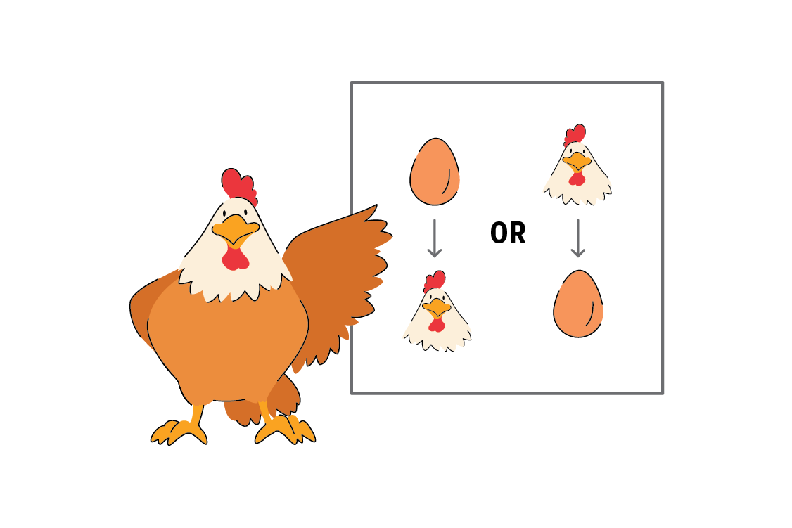
Very many things display correlation. The rooster crows when the sun rises.[6] The lights turn off when you flick a switch. Global temperatures have risen alarmingly since the 1800s, and meanwhile pirate numbers have dwindled to almost nothing.[7]
These examples show us that while correlation can appear as a result of causation, as in the case of the light switch, correlation certainly does not always imply causation, as in the case of the pirates.
Correlated things are not always related.[8] It’s possible to find many correlations with no readily imaginable causal interaction. The internet treasure Spurious Correlations collects many amusing examples of this. These spurious correlations most likely arise as a result of small sample size and coincidences that are bound to happen when making many comparisons. We should not be surprised if we find something that has low probability if we try many combinations.
In real world systems, spurious correlations can be cause for serious ethical concerns. For instance, certain characteristics may be spuriously associated with individuals or minority groups, and these characteristics may be highly predictive. As such, the model weights them as important during a learning task. This can easily embed bias and unfairness into an algorithm based on the spurious correlations in a given dataset.
The Principle of Common Cause
In a posthumous 1956 book, The Direction of Time, Hans Reichenbach outlined the principle of common cause. He states the principle this way:
“If an improbable coincidence has occurred, there must exist a common cause.”
Our understanding of causality has evolved, but this language is remarkably similar to what we use now. Let’s discuss how correlation may arise from causation.
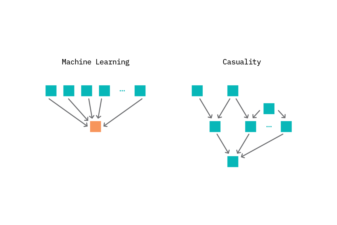
We will do this in the framework of Structural Causal Models (SCMs). An SCM is a directed acyclic graph of relationships between variables. The nodes represent variables, and the edges between them point from cause to effect. The value of each variable depends only on its direct parents in the graph (the other variables which point directly into it) and a noise variable that encapsulates any environmental interactions we are not modeling. We will examine three fundamental causal structures.
Causal Terminology
A causal graph is a directed acyclic graph denoting the dependency between variables.
A structural causal model carries more information than a causal graph alone. It also specifies the functional form of dependencies between variables.
Remarkably, it’s possible to do much causal reasoning - including a calculation of the size of causal effects - via the graph alone, without specifying a parametric form for the relationships between causes and effects.
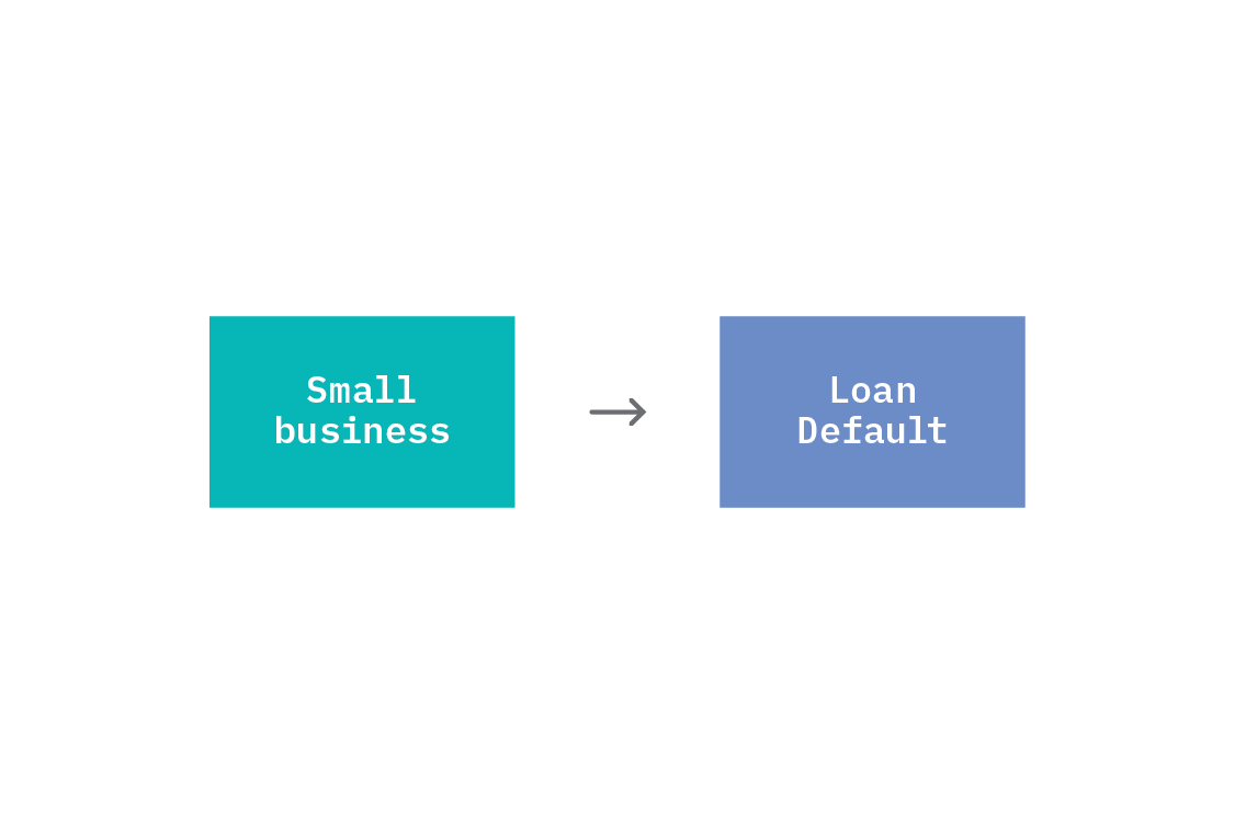
1. Direct causation
The simplest way in which correlation between two variables arises is when one variable is a direct cause of the other. We say that one thing causes another when a change in the first thing, while holding everything else constant, results in a change in the second. In the business loan defaulting example discussed earlier, we could create a two node graph with one of the nodes being whether or not a business is small (say “small business” with values 0 or 1) and the other node being “default” indicating whether or not the business defaulted on the loan. In this case, we would expect that a small business increases the chances of it defaulting.
This setup is immediately reminiscent of supervised learning, where we have a dataset of features, X, and targets, Y, and want to learn a mapping between them. However, in machine learning, we typically start with all available features and select those that are most informative about the target. When drawing a causal relationship, only those features we believe have an actual causal effect on the target should be included as direct causes. As we will see below, there are other diagrams that can lead to a predictive statistical relationship between X and Y in which neither directly causes the other.
2. Common cause
A common pattern is for a single variable to be the cause of multiple other variables. If a variable, Z, is a direct cause of both X and Y, we say that Z is a common cause and call the structure a “fork.” For example, unemployment could potentially cause both loan default and reduced consumer spend.
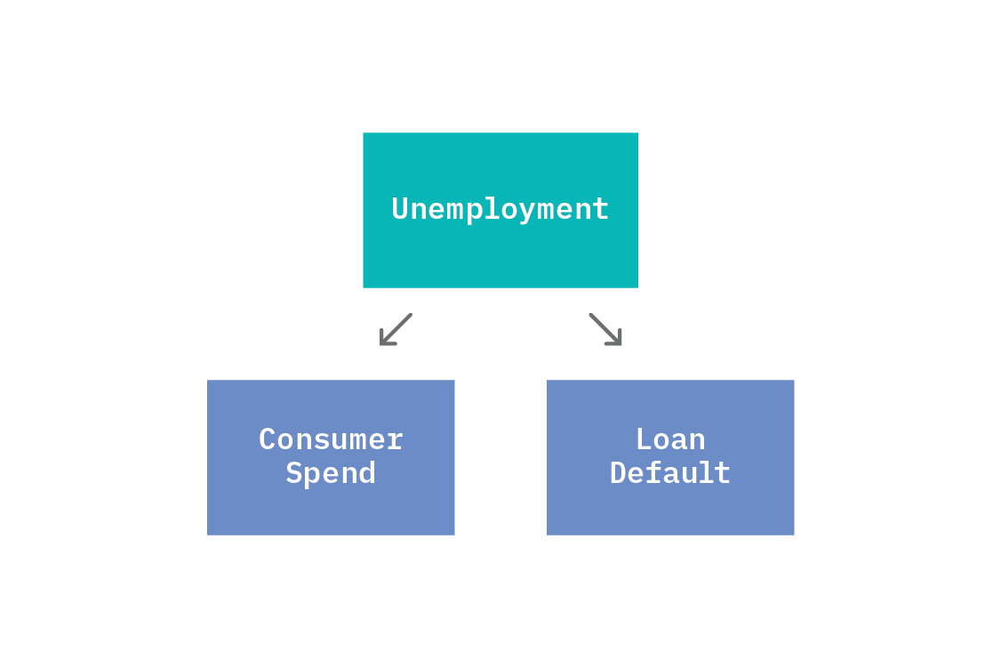
Because both consumer spend and loan default depend on unemployment, they will appear correlated. A given value of unemployment will generate some values of consumer spend and loan default, and when unemployment changes, both consumer spend and loan default will change. As such, in the joint distribution of the SCM, the two dependent variables (consumer spend and loan default) will appear statistically related to one another.
However, if we were to condition on unemployment (for instance, by selecting data corresponding to a fixed unemployment rate), we would see that consumer spend and loan default are independent from one another.
The common cause unemployment confounds the relationship between consumer spend and loan default. We are unable to correctly calculate the relationship between consumer spend and loan default without accounting for unemployment (by conditioning). This is especially dangerous if unnoticed.
Unfortunately, confounders can be tricky or impossible to detect from observational data alone. In fact, if we look only at consumer spend and loan default, we could see the same joint distribution as in the case where consumer spend and loan default are directly causally related. As such, we should think of causal graphs as encoding our assumptions about the system we are studying. We return to this point in How do we know which graph to use?
3. Common effect
The opposite common pattern is for one effect to have multiple direct causes. A node that has multiple causal parents is called a “collider” with respect to those nodes.
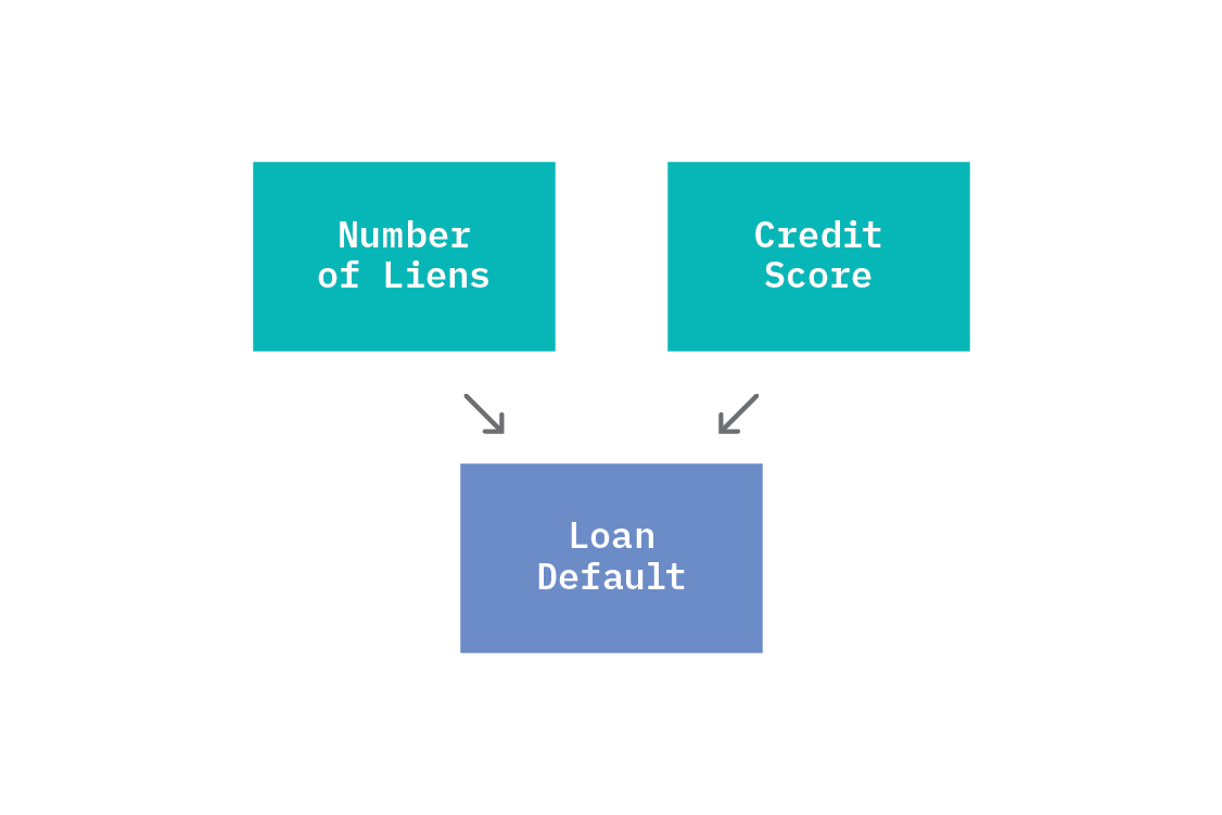
A collider is a node that depends on more than one cause. In this example, loan defaulting depends on both commercial credit score and number of liens (a “lien” refers to the right to keep possession of property belonging to another entity until a debt owed by that entity is discharged), so we call loan default a collider.
Colliders are different to chains of direct causation and forks because the conditioning behaviour works oppositely. Before any conditioning, commercial credit score and number of liens are unconditionally independent. There is no variable with causal arrows going into both commercial credit score and number of liens, and no arrow linking them directly, so we should not expect a statistical dependency. However, if we condition on the collider, we will induce a conditional dependence between commercial credit score and number of liens.
This may seem a bit unintuitive, but we can make sense of it with a little thought experiment. Loan default depends on both commercial credit score and number of liens, so if either of those changes value, the chance of loan default changes. We fix the value of loan default (say, we look only at those loans that did default). Now, if we were to learn anything about the value of commercial credit score, we would know something about the number of liens too; only certain values of number of liens are compatible with the conditioned value of loan defaulting and observed value of commercial credit score. As such, conditioning on a collider induces a spurious correlation between the parent nodes. Conditioning on a collider is exactly selection bias!
Structural Causal Models, in code
The small causal graphs shown above are an intuitive way to reason about causality. Remarkably, we can do much causal reasoning (and calculate causal effects) with these graphs, simply by specifying qualitatively which variables causally influence others. In the real world, causal graphs can be large and complex.
Of course, there are other ways to encode the information. Given the graph, we can easily write down an expression for the joint distribution: it’s the product of probability distributions for each node conditioned on its direct causal parents. In the case of a collider structure, x → z ← y, the joint distribution is simply p(x,y,z) = p(x) p(y) p(z|x,y). The conditional probability p(z|x,y) is exactly what we’re used to estimating in supervised learning!
If we know more about the system, we can move from this causal graph to a full structural causal model. An example SCM compatible with this graph would be:
from numpy.random import randn

def x():
  return -5 + randn()

def y():
  return 5 + randn()

def z(x, y):
  return x + y + randn()

def sample():
  x_ = x()
  y_ = y()
  z_ = z(x_, y_)
  return x_, y_, z_
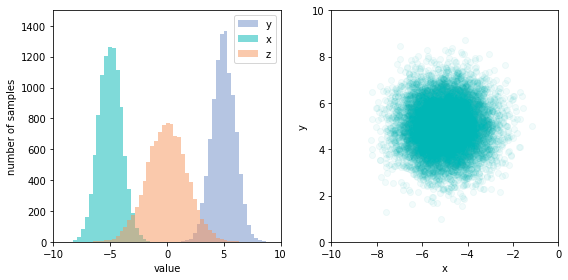
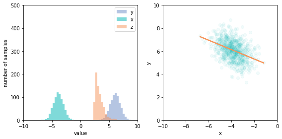
Each of the variables has an independent random noise associated with it, arising from factors not modeled by the graph. These distributions need not be identical, but must be independent. Notice that the structure of the graph encodes the dependencies between variables, which we see as the function signatures. The values of x and y are independent, but z depends on both. We can also see clearly that the model defines a generative process for the data, since we can easily sample from the joint distribution by calling the sample function. Doing so repeatedly allows us to chart the joint distribution, and see that x and y are indeed independent; there’s no apparent correlation in the scatter chart.
Now that we have a model in code, we can see a selection bias effect. If we condition the data to only values of z (the collider node) greater than a cutoff (which we can do easily, if inefficiently, by filtering the samples to those where z > 2.5), the previously independent x and y become negatively correlated.
From prediction to intervention
Now that we have some understanding of what a causal model is, we can get to the heart of causality: the difference between an observation and an intervention.
When we introduced the ladder of causation, we mentioned the notion of intervention, something that changes the system. This is a fundamental operation, and it is important to understand the difference between intervention and observation. It may not at first seem natural to consider intervening as a fundamental action, evoking a similar sense of confusion to when one first encounters priors in Bayesian statistics. Is an intervention subjective? Who gets to define what an intervention is?
Simply, an intervention is a change to the data generating process. Samples from the joint distribution of the variables in the graph may be obtained by simply “running the graph forward.” For each cause, we sample from its noise distribution and propagate that value through the SCM to calculate the resulting effects. To compute an interventional distribution, we force particular causes (on which we are intervening) to some value, and propagate those values through the equations of the SCM. This introduces a distribution different from the observational distribution with which we usually work.
There is sometimes confusion between an interventional distribution and a conditional distribution. A conditional distribution is generated by filtering an observed distribution to meet some criteria. For instance, we might want to know the loan default rate among the businesses to which we have granted a loan at a particular interest rate. This interest rate would itself likely have been determined by some model, and as such, the businesses with that rate will likely share statistical similarities.
The interventional distribution (when we intervene on interest rate) is fundamentally different. It is the distribution of loan defaulting if we fix the interest rate to a particular value, regardless of other features of the business that may warrant a different rate. This corresponds to removing all the inbound arrows to the interest rate in the causal graph; we’re forcing the value, so it no longer depends on its causal parents.
Clearly, not all interventions are physically possible! While we could intervene to set the interest rate, we of course would not be able to make every business a large one.
Interventions in code
It is easy to make interventions concrete with code. Returning to the collider example, to compute an interventional distribution, we could define a new sampling function where instead of drawing all variables at random, we intervene to set x to a particular value. Because this is an intervention, not simply conditioning (as earlier), we must make the change, then run the data generating process again.
def sample_intervened():
  x_ = -3
  y_ = y()
  z_ = z(x_, y_)
  return x_, y_, z_
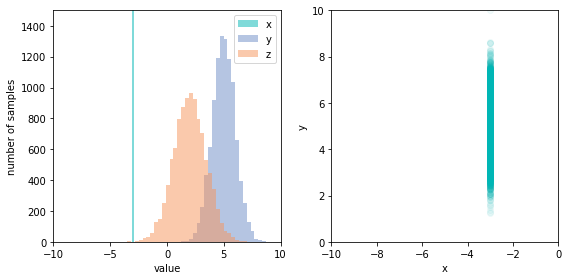
Performing this intervention results in a new distribution for z, which is different from the observational distribution that we saw earlier. Further, the relationship between x and y has changed; the joint distribution is now simply the marginal distribution of y, since x is fixed. This is a strikingly different relationship than when we simply conditioned the observational distribution.
Interventions in customer churn
In our interpretability report, we present a customer churn modeling use case. Briefly, given 20 features of the customers of a telco - things like tenure, demographic attributes, whether they have phone and internet services, and whether they have tech support - we must model their likelihood of churning within a fixed time. To do this, we turn to a dataset of customers and whether they churned in the time period. This can be modeled as straightforward binary classification, and we can use the resulting output scores as a measure of how likely a customer is to churn.
The model used to calculate the churn score is an ensemble of a linear model, a random forest, and a simple feed forward neural network. With appropriate hyperparameters and training procedure, such an ensemble is capable of good predictive performance. That performance is gained by exploiting subtle correlations in the data.
To understand the predictions made, we apply LIME. This returns a feature importance at the local level: which features contributed to each individual prediction. To accompany the analysis, we built Refractor, an interface for exploring the feature importances. Examining these is interesting, and highlights the factors that are correlated with a customer being likely to churn. Refractor suggests which features most affect the churn prediction, and allows an analyst to change customer features and see the resulting churn prediction.
Because we have a model that provides new predictions when we change the features, it is tempting to believe we can infer from this alone how to reduce churn probability. Aside from the fact that often the most important features cannot be changed by intervention (tenure, for instance), this is an incorrect interpretation of what LIME and our model provide. The correct interpretation of the prediction is the probability of churn for someone who naturally occurred in our dataset with those features, or, for instance, what this same customer’s churn probability will look like next year (when tenure will have naturally increased by one year), assuming none of their other features change.
Of course, there are some features that can be changed in reality. For instance:
- the telco could reduce the monthly fee for a customer, or
- try to convince them to change contract type from monthly to yearly (one does not have to think too hard about why this changes the short-term churn probability), or
- upgrade the service from DSL to fiber-optic.
Which of these interventions would most decrease the probability that the customer churns? We don’t know. Our model alone - for all its excellent predictive accuracy - can’t tell us that, precisely because it is entirely correlative. Even a perfect model, that 100% accurately predicts which customers will churn, cannot tell us that.
With some common sense, we can see that a causal interpretation is not appropriate here. LIME often reports that having a faster fiber-optic broadband connection increases churn probability, relative to slower DSL. It seems unlikely that faster internet has this effect. In reality, LIME is correctly reporting that there is a correlation between having fiber-optic and churning, likely because of some latent factors - perhaps people who prefer faster internet are also intrinsically more willing to switch providers. This distinction of interpretation is crucial.
The model can only tell us what statistical dependencies exist in the dataset we trained it on. The training dataset was purely observational - a snapshot of a window of time with observations about those customers in it. If we select “give the customer access to tech support” in the app, the model can tell us that similar customers who also had access to tech support were less likely to churn. Our model only captures information about customers who happened to have some combination of features. It does not capture information about what happens when we change a customer’s features. This is an important distinction.
To know what would happen when we intervene to change a feature, we must compute the interventional distribution (or a point prediction), which can be very different from the observational distribution. In the case of churn, it’s likely the true causal graph is rather complex.
Interpretability techniques such as LIME provide important insights into models, but they are not causal insights. To make good decisions using the output of any interpretability method, we need to combine it with causal knowledge.
Often, this causal knowledge is not formally specified in a graph, and we simply call it “domain knowledge,” or expertise. We have emphasized what the model cannot do, in order to make the technical point clear, but in reality, anyone working with the model would naturally apply their own expertise. The move from that to a causal model requires formally encoding the assumptions we make all the time and verifying that the expected statistical relationships hold in our observed data (and if possible, experimenting). Doing so would give us an understanding of the cause-effect relationships in our system, and the ability to reason quantitatively about the effect of interventions.
Constructing a useful causal model of churn is a complex undertaking, requiring both deep domain knowledge and a detailed technical understanding of causal inference.[9] In Causality and Invariance, we will discuss some techniques that are bridging the gap between a full causal model and the supervised learning setup we use in problems like churn prediction.
When do we need interventions?
When do we need to concern ourselves with intervention and causality? If all we want to do is predict, and to do so with high accuracy (or whatever model performance metric we care about), then we should use everything at our disposal to do so. That means making use of all the variables that may correlate with the outcome we’re trying to predict, and it doesn’t matter that they don’t cause the outcome. Correlation is not causation, but correlation is still predictive,[10] and supervised learning excels at discovering subtle correlations.
Some situations in which this pure supervised learning approach is useful:
- We want to predict when a machine in our factory will fail.
- We want to forecast next quarter’s sales.
- We want to identify named entities in some text.
Conversely, if we want to predict the effect of an intervention, we need causal reasoning. For example:
- We want to know what to change about our machines to reduce the likelihood of failures.
- We want to know how we can increase next quarter’s sales.
- We want to know whether longer or shorter article headlines generate more clicks.[11]
How do we know which graph to use?
Knowing the true causal structure of a problem is immensely powerful. Earlier in this chapter, we discussed three building blocks of causal graphs (direct causation, forks, and colliders) but for real problems, a graph can be arbitrarily complex.
The graph structure allows us to reason qualitatively about what statistical dependencies ought to hold in our data. In the absence of abundant randomized controlled trials or other experiments, qualitative thinking is necessary for causal inference. We must use our domain knowledge to construct a plausible graph to test against the data we have. It is possible to refute a causal graph by considering the statistical independence relations it implies, and matching those against the expected relations from the causal structure. For example, if two variables are connected by a common cause on which we have not conditioned, we should expect a statistical dependence between them.
Causal Discovery
The independence relationships implied by a graph can be used for causal discovery. Causal discovery is the process of attempting to recover causal graphs from observational data. There are many approaches appropriate for different sets of assumptions about the graph. However, since many causal graphs can imply the same joint distribution, the best we should hope for from causal discovery is a set of plausible graphs, which, if we are fortunate, may contain the true graph. In reality, inferring the direction of causation in even a two variable system is not always possible from data alone.[12]
It is not, in general, possible to prove a causal graph, since different graphs can result in the same observed and even interventional distributions. The difficulty of confirming a causal relationship means that we should always proceed with caution when making causal claims. It is best to think of causal models as giving results conditional on a set of causal assumptions. Two nodes that are not directly connected in the causal graph are assumed to be independent in the data generating process, except insofar as the causal relations described above (or combinations of them) induce a statistical dependence.
The validity of the results depends on the validity of the assumptions. Of course, we face the same situation in all machine learning work - and it is to be expected that stronger, causal claims require stronger assumptions than merely observational claims.
One case in which we may be able to write down the true causal graph is when we have ourselves created the system. For instance, a manufacturing line may have a sufficiently deterministic process that makes it possible to write down a precise graph encoding which parts move from which machine to another. If we were to model the production of faulty parts, that graph would be a good basis for the causal graph, since a machine that has not processed a given faulty part is unlikely to be responsible for the fault, and causal graphs encode exactly these independences.
TL;DR
Causal graphical models present an intuitive and powerful means of reasoning about systems. If an application requires only pure prediction, this reasoning is not necessary, and we may apply supervised learning to exploit subtle correlations between variables and our predicted quantity of interest. However, when a prediction will be used to inform a decision that changes the system, or we want to predict for the system under intervention, we must reason causally - or else likely draw incorrect conclusions. That said, behind every causal conclusion there is always a causal assumption that cannot be tested or verified by mere observation.
Even without a formal education in causal inference, there are advantages to the qualitative reasoning enabled by causal graphical models. Trying to write down a causal graph forces us to confront our mental model of a system, and helps to highlight potential statistical and interpretational errors. Further, it precisely encodes the independence assumptions we are making. However, these graphs could be complex and high dimensional and require close collaboration between practitioners and domain experts who have substantive knowledge of the problem.
In many domains, problems such as the large numbers of predictors, small sample sizes, and possible presence of unmeasured causes, remain serious impediments to practical applications of causal inference. In such cases, there is often limited background knowledge to reduce the space of alternative causal hypotheses. Even when experimental interventions are possible, performing the many thousands of experiments that would be required to discover causal relationships between thousands or tens of thousands of predictors is often not practical.
Given these challenges, how do we combine causal inference and machine learning? Many of the researched approaches at the intersection of ML and causal inference are motivated by the ability to apply causal inference techniques to high dimensional data, and in domains where specifying causal relationships could be difficult. In the next chapter, we will bridge this gap between structural causal models and supervised machine learning.
Causality and Invariance
Supervised machine learning is very good at prediction, but there are useful lessons we can take from causal models even for purely predictive problems.
Relative to recent advancements made in the broader field of machine learning, the intersection of machine learning and causal reasoning is still in its infancy. Nonetheless, there are several emerging research directions. Here, we focus on one particularly promising path: the link between causality and invariance. Invariance is a desirable property for many machine learning systems: a model that is invariant is one that performs well in new circumstances, particularly when the underlying data distribution changes. As we will see in this chapter, invariance also provides a route to some causal insights, even when working only with observational data.
The great lie of machine learning
In supervised learning, we wish to predict something that we don’t know, based on only the information that we do have. Usually, this boils down to learning a mapping between input and output.
To create that map, we require a dataset of input features and output targets; the number of examples required scales with the complexity of the problem. We can then fit the parameters of a learning algorithm to the dataset to minimize some loss function that we choose. For instance, if we are predicting a continuous number, like temperature, we might seek to minimize the mean squared difference between the prediction and the true measurements.
If we are not careful, we will overfit the parameters of the ML algorithm to the dataset we train on. In this context, an overfit model is one that has learned the idiosyncrasies (the spurious correlations!) of our dataset. The result is that when the model is applied to any other dataset (even one with the same data generating process), the model’s performance is poor, because it is relying on superficial features that are no longer present.
To avoid overfitting, we employ various regularization schemes and adjust the capacity of the model to an appropriate level. When we fit the model, we shuffle and split our data, so we may learn the parameters from one portion of the data, and validate the resulting model’s performance on another portion. This gives us confidence that the learned parameters are capturing something about all the data we have, and not merely a portion of it.
Whatever procedure we use (be it cross-validation, forward chaining for time series, or simpler train-test-validation splits), we are relying on a crucial assumption. The assumption is that the data points are independent and identically distributed ( i.i.d.). By independent, we mean that each data point was generated without reference to any of the others, and by identically distributed, we mean that the underlying distributions in the data generating process are the same for all the data points.
Paraphrasing Zoubin Ghahramani,
the i.i.d. assumption is the great lie of machine learning.
Rarely are data truly independent and identically distributed. What are the ramifications of this misassumption for machine learning systems?
Dangers of spurious correlations
When we train a machine learning system with the i.i.d. assumption, we are implicitly assuming an underlying data generating process for that data. This data generating process defines an environment. Different data generating processes will result in different environments, with different underlying distributions of features and targets.
When the environment in which we predict differs from the environment in which our machine learning system was trained, we should expect it to perform poorly. The correlations between features and the target are different - and, as such, the model we created to map from features to target in one environment will output incorrect values of the target for the features in another environment.
Unfortunately, it’s rarely possible to know whether the data generating process for data at predict time (in a deployed ML system, for instance) will be the same as during training time. Even once the system is predicting in the wild, if we do not or cannot collect ground truth labels to match to the input features on which the prediction was based, we may never know.
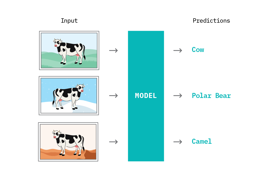
This problem is not academic. Recognition in Terra Incognita points this out in humorous fashion (see also Unbiased Look at Dataset Bias). Both of these papers highlight that computer vision systems trained for visual recognition of objects, animals, and people can utterly fail to recognise the same objects in different contexts. A cow on the slopes of an alpine field is easily recognised, but a cow on a beach is not noticed at all, or poorly classified as a generic “mammal.”
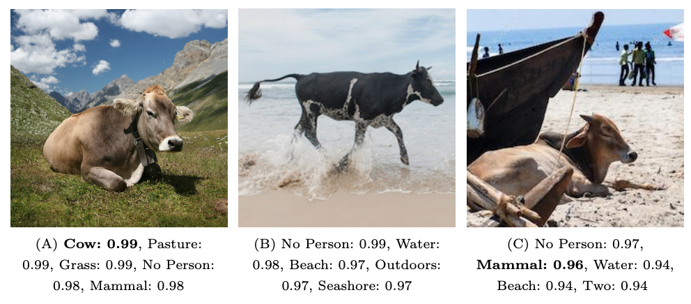
These failures should not come as a surprise to us! Supervised machine learning is designed to exploit correlations between features to gain predictive performance, and cows and alpine pastures are highly correlated. Neural networks are a very flexible class of models that encode the invariants of the dataset on which they’re trained. If cows dominantly appear on grass, we should expect this to be learned.
When is a correlation spurious?
In supervised learning, we learn to use subtle correlations, possibly in high dimensional spaces like natural images, to make predictions. What distinguishes a genuine correlation from a spurious one? The answer depends on the intended use of the resulting model.
If we intend for our algorithm to work in only one environment, with very similar images, then we should use all the correlations at our disposal, including those that are very specific to our environment. However, if - as is almost always the case - we intend the algorithm to be used on new data outside of the training environment, we should consider any correlation that only holds in the training environment to be spurious. A spurious correlation is a correlation that only appears to be true due to a selection effect (such as selecting a training set!).
In Background: Causal Inference, we saw that correlation can arise from several causal structures. In the strictest interpretation, any correlation that does not arise from direct causation could be considered spurious.
Unfortunately, given only a finite set of training data, it is often not possible to know which correlations are spurious. The methods in this section are intended to address precisely that problem.
When a machine learning algorithm relies heavily on spurious correlations for predictive performance, its performance will be poor on data from outside the dataset on which it was trained. However, that is not the only problem with spurious correlations.
There is an important and growing emphasis on interpretability in machine learning. A machine learning system should not only make predictions, but also provide a means of inspecting how those predictions were made. If a model is relying on spurious correlations, the feature importances (such as those calculated by LIME or SHAP) will be similarly spurious. No one should make decisions based on spurious explanations!
Invariance
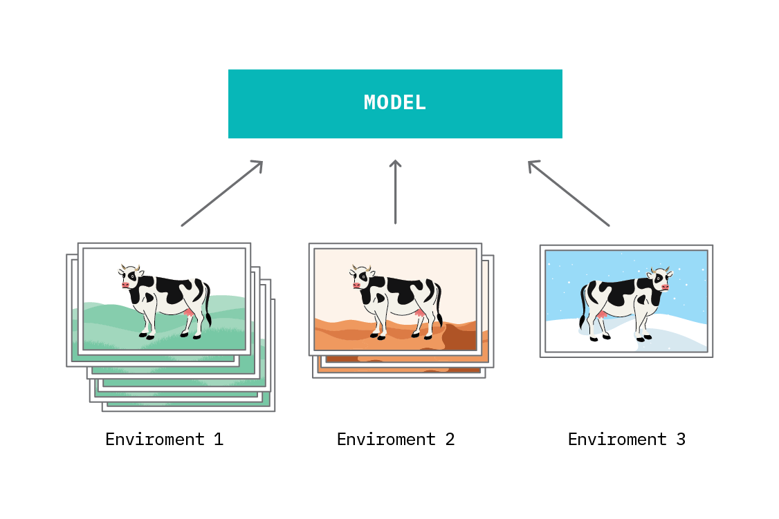
To be confident of our predictions outside of our training and testing datasets, we need a model that is robust to distributional shifts away from the training set. Such a model would have learned a representation which ignores dataset-specific correlations, and instead relies upon features that affect the target in all environments.
How can we go about creating such a model? We could simply train our model with data from multiple environments, as we often do in machine learning (playing fast and loose with the i.i.d. assumption). However, doing so naively would provide us with a model that can only generalize to the environments it has seen (and interpolations of them, if we use a robust objective).[13] We wish our model to generalize beyond the limited set of environments we can access for training, and indeed extrapolate to new and unseen (perhaps unforeseen) environments. The property we are looking for - performing optimally in all environments - is called invariance.
The connection between causality and invariance is well established. In fact, causal relationships are - by their nature - invariant. The way many intuitive causal relationships are established is by observing that the relationship holds all the time, in all circumstances.
Consider how physical laws are discovered. They are found by performing a series of experiments in different conditions, and monitoring which relationships hold, and what their functional form is. In the process of discovering nature’s laws, we will perform some tests that do not show the expected result. In cases where a law does not hold, this gives us information to refine the law to something that is invariant across environments.[14]
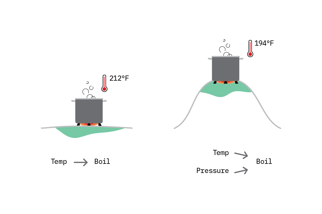
For example, water boils at 100° Celsius (212° Fahrenheit). We could observe that everywhere, and write a simple causal graph: temperature → water boiling. We have learned a relationship that is invariant across all the environments we have observed.
Then, a new experiment conducted on top of a tall mountain reveals that on the mountain, water boils at a slightly lower temperature. After some more experimentation, we improve our causal model, by realising that in fact, both temperature and pressure affect the boiling point of water, and the true invariant relationship is more complicated.
The mathematics of causality make the notion of invariance and environments precise. Environments are defined by interventions in the causal graph. Each intervention changes the data generating process, such that the correlations between variables in the graph may be different (see From prediction to intervention). However, direct causal relationships are invariant relationships: if a node in the causal graph depends only on three variables, and our causal model is correct, it will depend on those three variables, and in the same way, regardless of any interventions. It may be that an intervention restricts the values that the causal variables take, but the relationship itself is not changed. Changing the arguments to a function does not change the function itself.
Invariance and machine learning
In the machine learning setting, we are mostly concerned with using features to predict a target. As such, we tend to select features for their predictive performance. In contrast, causal graphs are constructed based on domain knowledge and statistical independence relations, and thus encode a much richer dependency structure. However, we are not always interested in the entire causal graph. We may be interested only in the causes of a particular target variable. This puts us closer to familiar machine learning territory.
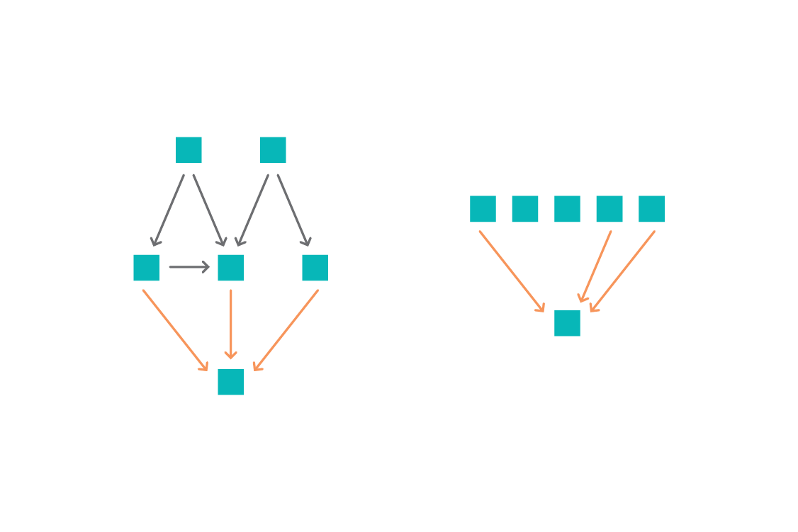
We will now examine two approaches to combining causal invariance and machine learning. The first, invariant causal prediction, uses the notion of invariance to infer the direct causes of a variable of interest. This restricted form of causal discovery (working out the structure of a small part of the graph in which we are interested) is appropriate for problems with well defined variables where a structural causal model (or at least causal graph) could be created - in principle, if not in practice.
Not all problems are amenable to SCMs. In the following section, we describe invariant risk minimization, where we forego the causal graph and seek to find a predictor that is invariant across multiple environments. We don’t learn anything about the graph structure from this procedure, but we do get a predictor with greatly improved out-of-distribution generalization.
Invariant Causal Prediction
Invariant causal prediction (ICP) addresses the task of invariant prediction explicitly in the framework of structural causal models.
Often, the quantity we are ultimately concerned with in a causal analysis is the causal effect of an intervention: what is the difference in the target quantity when another variable is changed?[15] To calculate that, we either need to hold some other variables constant, or else account for the fact that they have changed. If we are only interested in the causes that affect a particular target, we do not need to construct the whole graph, but rather only determine which factors are the true direct causes of the target. Once we know that, we can answer causal questions, like how strongly each variable contributes to the effect, or the causal effect of changing one of the input variables.
The key insight offered by ICP is that because direct causal relationships are invariant, we can use that to determine the causal parents (the direct causes). The set-up is similar to that of machine learning; we have some input features, and we’d like a model of an output target. The difference from supervised learning is that the goal is not “performance at predicting the target variable.” In ICP, we aim to discover the direct causes of a given variable - the variables that point directly into the target in the causal graph.
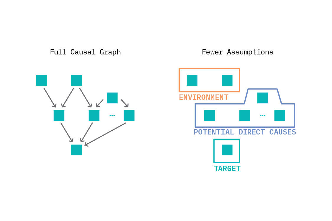
To use ICP, we take a target variable of interest, and construct a plausible list of the potential direct causes of that variable. Then we must define environments for the problem: each environment is a dataset. In the language of SCMs, each environment corresponds to data observed when a particular intervention somewhere in the graph was active. We can reason about this even without specifying the whole graph, or even which particular intervention was active, as long as we can separate the data into environments. In practice, we often take an observed variable to be the environment variable, when it could plausibly be so.
For instance, perhaps we are predicting sales volume in retail, and want to discern what store features causally impact sales. The target is sales volume, and the potential causes would be features like store size, number of nearby competitors, level of staffing, and so on.
Environments might be different counties (or even countries) - something that is unlikely to impact the sales directly, but which may impact the features that impact the sales. For instance, different places will have different populations, and population density is a possible cause of sales volume. Importantly, the environment cannot be a descendent of the target variable.[16]
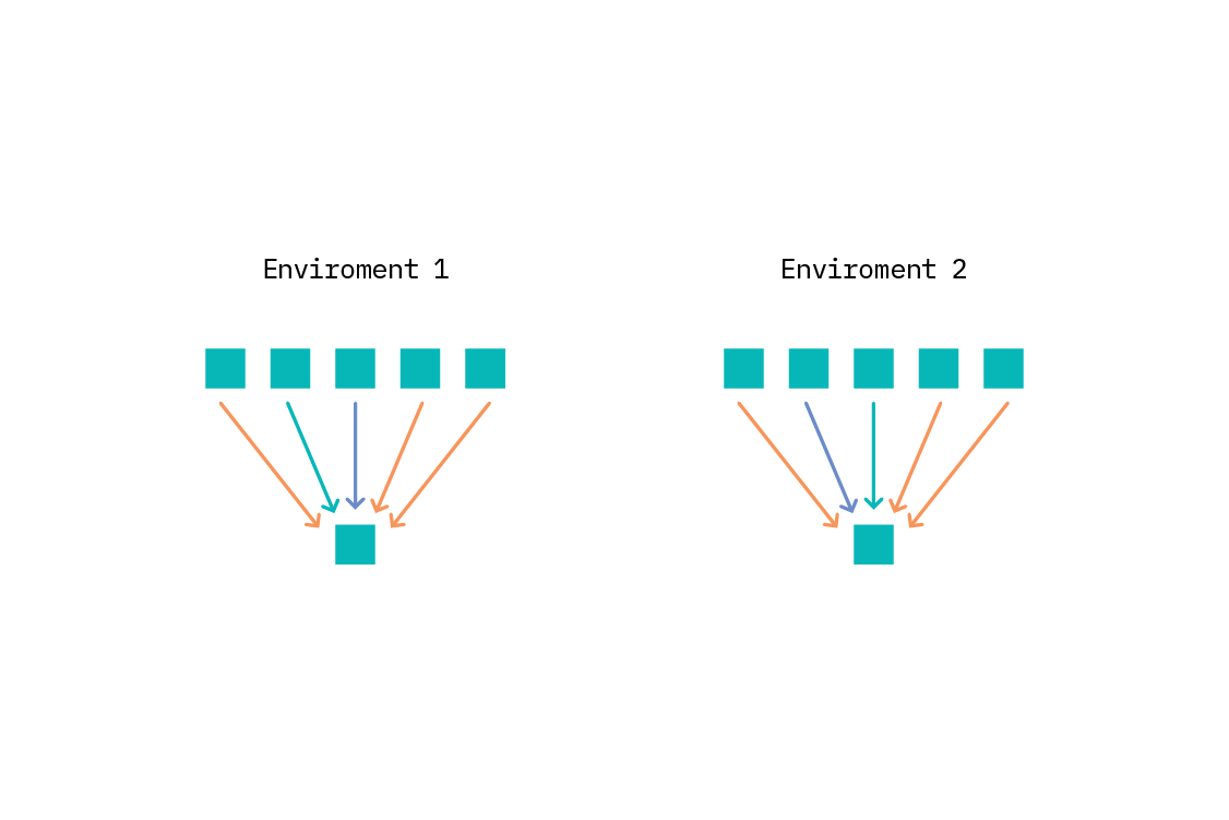
To apply ICP, we first consider a subset of features. We then fit a linear (Gaussian) regression from this subset to the target in each environment we have defined. If the model does not change between environments (which can be assessed either via the coefficients or a check on residuals), we have found a set of features that appear to result in an invariant predictor. We iterate over subsets of features combinatorially. Features that appear in a model that is invariant are plausible causes of the target variable. The intersection of these sets of plausible causes (i.e., the features which are predictive in all environments) is then a subset of the true direct causes.
In machine learning terms, ICP is essentially a feature selection method, where the features selected are very likely to be the direct causes of the target. The model built atop those features can be interpreted causally: a high coefficient for a feature means that feature has a high causal effect on the target, and changes in those features should result in the predicted change in the target.
Naturally, there are some caveats and assumptions. In particular, we must assume there is no unobserved confounding between the features and the target (recall that a confounder is a common cause of the feature and target). If there are known confounders, we must make some adjustments to account for them, as detailed in the ICP paper. The authors provide an R package, InvariantCausalPrediction, implementing the methods.
The restriction of using a linear Gaussian model - and that environments be discrete, rather than defined by the value of a continuous variable - are removed by nonlinear ICP.[17] In the nonlinear case, we replace comparing residuals or coefficients with conditional independence tests.[18]
Invariant Risk Minimization
When using Invariant Causal Prediction, we avoid writing the full structural causal model, or even the full graph of the system we are modeling, but we must still think about it.
For many problems, it’s difficult to even attempt drawing a causal graph. While structural causal models provide a complete framework for causal inference, it is often hard to encode known physical laws (such as Newton’s gravitation, or the ideal gas law) as causal graphs. In familiar machine learning territory, how does one model the causal relationships between individual pixels and a target prediction? This is one of the motivating questions behind the paper Invariant Risk Minimization (IRM). In place of structured graphs, the authors elevate invariance to the defining feature of causality.
They also make the connection between invariance and causality well:
“If both Newton’s apple and the planets obey the same equations, chances are that gravitation is a thing.” – IRM authors
Like ICP, IRM uses the idea of training in multiple environments. However, unlike ICP, IRM is not concerned with retrieving the causal parents of the target in a causal graph. Rather, IRM focusses on out-of-distribution generalization: the performance of a predictive model when faced with a new environment. The technique proposed aims to create a data representation, on which a classifier or regressor can perform optimally in all environments. The paper itself describes the IRM principle:
“To learn invariances across environments, find a data representation such that the optimal classifier on top of that representation matches for all environments.” – IRM authors
Said differently, the idea is that there is a latent causal structure behind the problem we’re learning, and the task is to recover a representation that encodes the part of that structure that affects the target. This is different from selecting features, as in Invariant Causal Prediction. In particular, it provides a bridge from very low level features (such as individual pixels) to a representation encoding high level concepts (such as cows).
The causal direction
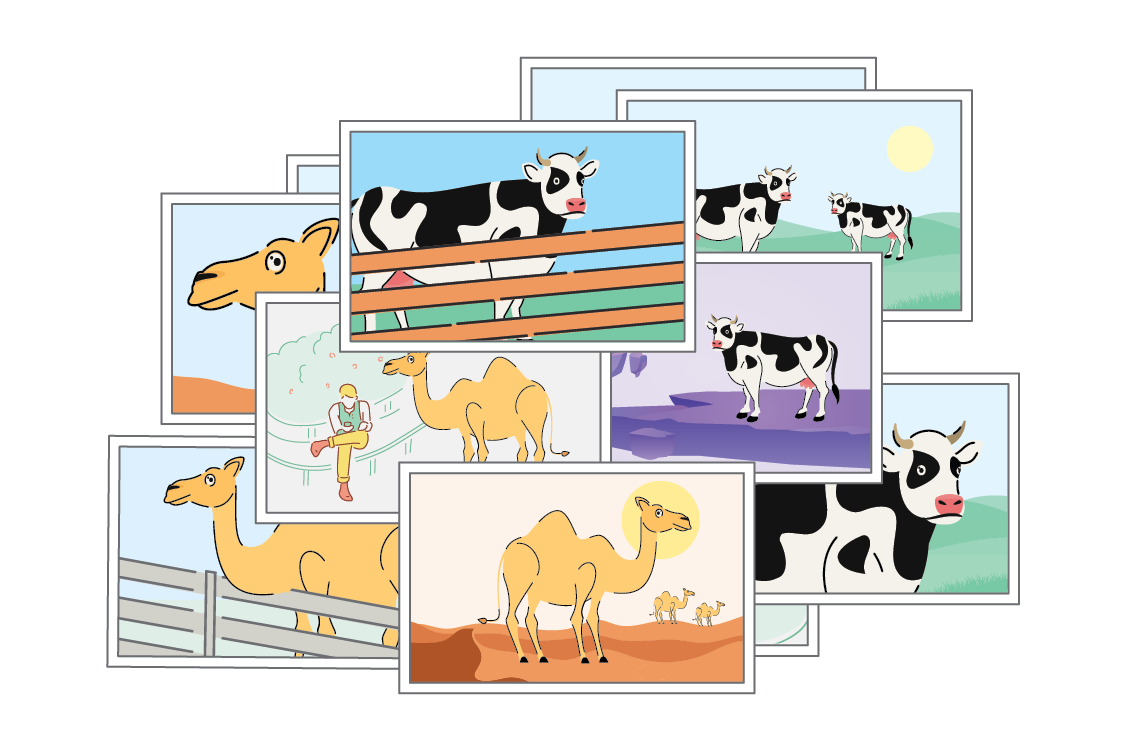
The idea of a latent causal system generating observed features is particularly useful as a view of computer vision problems. Computer vision researchers have long studied the generative processes involved in moving from real world objects to pixel representations.[19] It’s instructive to inspect the causal structure of a dataset of cow pictures.
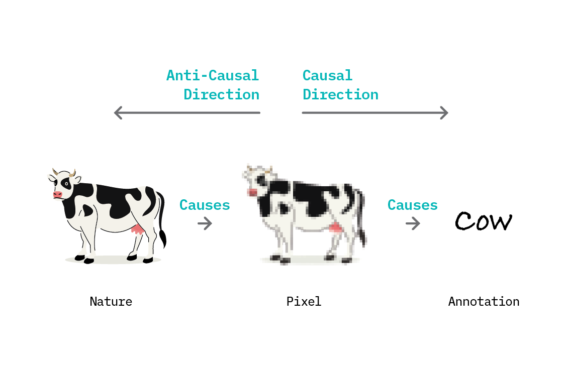
In nature, cows exist in fields and on beaches, and we have an intuitive understanding that the cow itself and the ground are different things. A neural network trying to predict the presence of a cow in an image could be called an “anti-causal” learning problem, because the direction of causation is the opposite of the direction of prediction. The presence of a cow causes certain pixel patterns, but pixels are the input to the network, and the presence of a cow is the output.
However, a further sophistication can be added: the dataset on which we train a neural network is not learning from nature, but rather from annotations provided by humans. This changes the causal direction: we are now learning the effect from the cause, since those annotations are caused by the pixels of the image. This is the view taken by IRM,[20] which thus interprets supervised learning from images as being a causal (rather than anti-causal) problem.[21]
Not all supervised learning problems are causal. Anti-causal supervised learning problems arise when the label is not provided based on the features, but by some other mechanism that causes the features. For example, in medical imaging, we could obtain a label without reference to the image itself by observing the case over time (this is not a recommended approach for treatment, of course).
Learning in the causal direction explains some of the success of supervised learning - there is a chance that it can recover invariant representations without modification. Any supervised learning algorithm is learning how to combine features to predict the target. If the learning direction is causal, each input is a potential cause of the output, and it’s possible that the features learned will be the true causes. The modifications that invariant risk minimization makes to the learning procedure improve the chance by specifically promoting invariance.
How IRM works
To learn an invariant predictor, we must provide the IRM algorithm with data from multiple environments. As in ICP, these environments take the form of datasets - and, as such, the environments must be discrete. We need not specify the graphical or interventional structure associated with the environments. The motivating example of the IRM paper asks us to consider a machine learning system to distinguish cows from camels, highlighting a similar problem to that which Recognition in Terra Incognita does: animals being classified based on their environment, rather than on the animal itself. In this case, cows on sand may be misclassified as camels, due to the spurious correlations absorbed by computer vision systems.
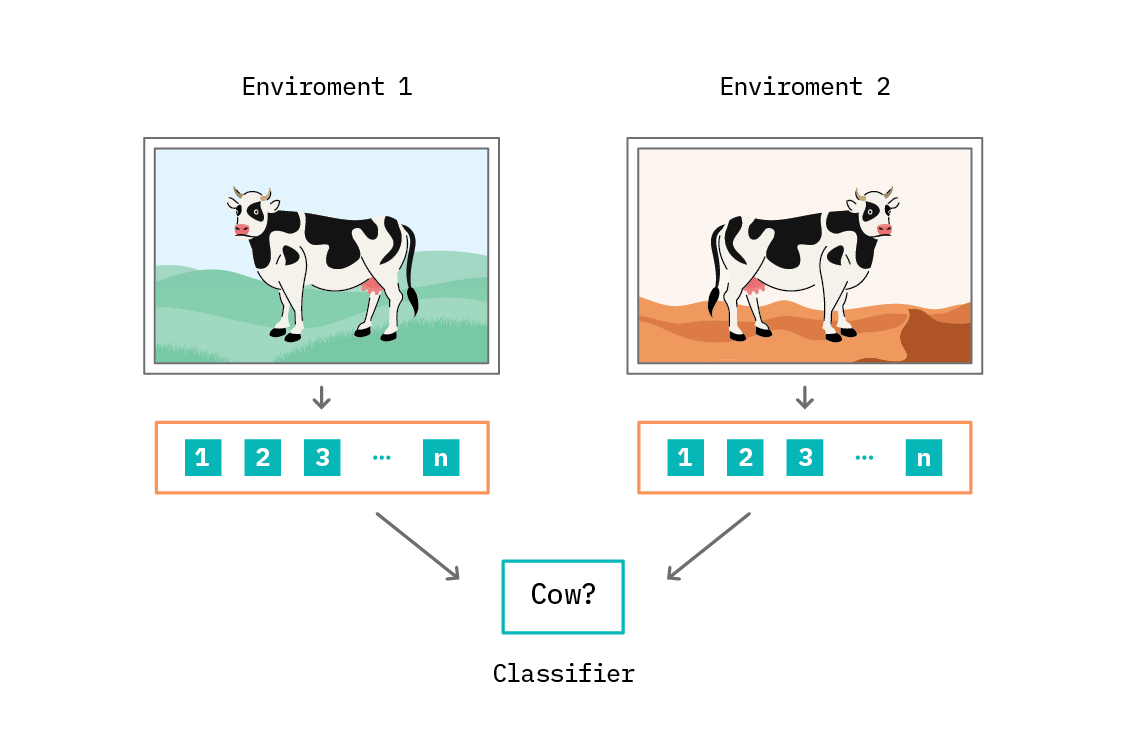
Simply providing data from multiple environments is not enough. The problem of learning the optimal classifier in multiple environments is a bi-level constrained optimization problem, in which we must simultaneously find the optimal data representation and optimal classifier across multiple separate datasets. IRM reduces the problem to a single optimization loop, with the trick of using a constant classifier and introducing a new penalty term to the loss function.
IRM loss = sum over environments (error + penalty)
The error is the usual error we would use for the problem at hand - for example, the cross entropy for a classification problem - calculated on each environment. The technical definition of the new penalty term is the squared gradient norm with respect to a constant classifier, but it has an intuitive explanation. While the error measures how well the model is performing in each environment, the penalty measures how much the performance could be improved in each environment with one gradient step.
By including the penalty term in the loss, we punish high gradients (situations in which a large improvement in an environment would be possible with one more epoch of learning). The result is a model with optimal performance in all environments. Without the IRM penalty, a model could minimize the loss by performing extremely well in just one environment, and poorly in others. Adding a term to account for the model having a low gradient (roughly, it has converged) in each environment ensures that the learning is balanced between environments.
To understand the IRM paradigm, we can perform a thought experiment. Imagine we have a dataset of cows and camels, and we’d like to learn to classify them as such. We separate out the dataset by the geolocation of photos - those taken in grassy areas form one environment, and those taken in deserts form another.
As a baseline, we perform regular supervised learning to learn a binary classifier between cows and camels. The learning principle at work in supervised learning is referred to as empirical risk minimization, (ERM); we’re just seeking to minimize the usual cross-entropy loss.[22] We’ll surely find that we can get excellent predictive performance on these two environments, because we have explicitly provided data from both.
The trouble arises when we want to identify a cow on snow, and find that our classifier did not really learn to identify a cow; it learned to identify grass. The holdout performance of our model in any new environment we haven’t trained on will be poor.
With IRM, we perform the training across (at least) two environments, and include the penalty term for each in the loss. We’ll almost certainly find that our performance in the training environments is reduced. However, because we have encouraged the learning of invariant features that transfer across environments, we’re more likely to be able to identify cows on snow. In fact, the very reason our performance in training is reduced is that we’ve not absorbed so many spurious correlations that would hurt prediction in new environments.
It is impossible to guarantee that a model trained with IRM learns no spurious correlations. That depends entirely on the environments provided. If a particular feature is a useful discriminator in all environments, it may well be learned as an invariant feature, even if in reality it is spurious. As such, access to sufficiently diverse environments is paramount for IRM to succeed.
However, we should not be reckless in labeling something as an environment. Both ICP and IRM note that splitting on arbitrary variables in observational data can create diverse environments while destroying the very invariances we wish to learn. While IRM promotes invariance as the primary feature of causality, it pays to hold a structural model in the back of one’s mind, and ask if an environment definition makes sense as something that would alter the data-generating process.
Considerations for applying IRM
IRM buys us extrapolation powers to new datasets, where independent and identically distributed supervised learning can (at best) interpolate between them. Using IRM to construct models improves their generalization properties by explicitly promoting performance across multiple environments, and leaves us with a new, closer-to-causal representation of the input features. Of course, this representation may not be perfect (IRM is an optimization-based procedure, and we will never know if we have found the true minimum risk across all environments) but it should be a step towards latent causal structure. This means that we can use our model to predict based on true, causal correlations, rather than spurious, environment-specific correlations.
However, there is no panacea, and IRM does come with some challenges.
Often, the dataset that we use in a machine learning project is collected well ahead of time, and may have been collected for an entirely different purpose. Even when a well-labeled dataset that is amenable to the problem exists, it is seldom accompanied by detailed metadata (by which we mean “information about the information”). As such, we often do not have information about the environment in which the data was collected.
Another challenge is finding data from sufficiently diverse environments. If the environments are similar, IRM will be unlikely to learn features that generalize to environments that are different. This is both a blessing and a curse - on the one hand, we do not need to have perfectly separated environments to benefit from IRM, but on the other hand, we are limited by the diversity of environments. If a feature appears to be a good predictor in all the environments we have, IRM will not be able to distinguish that from a true causal feature. In general, the more environments we have, and the more diverse they are, the better IRM will do at learning an invariant predictor, and the closer we will get to a causal representation.
No model is perfect, and whether or not one is appropriate to use depends on the objective. IRM is more likely to produce an invariant predictor, with good out-of-distribution performance, than empirical risk minimization (regular supervised learning), but using IRM will come at the expense of predictive performance in the training environment.
It’s entirely possible that for a given application, we may be very sure that the data in the eventual test distribution (“in the wild”) will be distributed in the same way as our training data. Further, we may know that all we want to do with the resulting model is predict, not intervene. If both these things are true, we should stick to supervised learning with empirical risk minimization and exploit all the spurious correlations we can.
Prototype
The promise of Invariant Risk Minimization (greatly improved out-of-distribution generalization using a representation that is closer-to-causal) is tempting. The IRM paper performs some experiments that clearly show the method works when applied to an artificial structural causal model. Further, an experiment in which an artificial spurious correlation is injected into the MNIST dataset (by coloring the images) is detailed, and works.
In order to gain a better understanding of the algorithm and investigate further, we wanted to test the same technique in a less artificial scenario: on a natural image dataset.
The Wildcam dataset
The iWildCam 2019 dataset (from The iWildCam 2019 Challenge Dataset) consists of wildlife images taken using camera traps. In particular, the dataset contains the Caltech Camera Traps (CCT) dataset, on which we focus. The CCT dataset contains 292,732 images, with each image labeled as containing one of 13 animals, or none. The images are collected from 143 locations, and feature a variety of weather conditions and all times of day. The challenge is to identify the animal present in the image.

Experimental setup
This setup maps naturally to the environmental splits used in IRM. Each camera trap location is a distinct physical environment which is roughly consistent, allowing for seasonal, weather, and day/night patterns. No two environments are the same, though the camera locations are spread around roughly the same geographic region (the American Southwest).
The objects of interest in the dataset are animals, which are basically invariant across environments: a raccoon looks like a raccoon in the mountains and in your backyard (though the particular raccoon may be different). The images are not split evenly between environments, since there is more animal activity in some places than others. Nor are the animal species evenly distributed among cameras. Some cameras will primarily produce images of one species or another, depending on the animals active in the area.
If we were to naively train a model using empirical risk on a subset of cameras, we could well end up learning exactly those class imbalances. If 99% of the images from camera 1 are labeled as deer, then we could have a 99% accurate classifier by learning to recognize the fallen tree that is present only in camera 1, rather than the deer themselves. Clearly such a classifier has not really learned to recognize deer, and would be useless for predicting in another environment.
We want to learn to recognize the animals themselves. The IRM setup seems ideally suited to address this challenge.
To validate the approach, we restricted our experiment to only three cameras and two animal species, which were randomly chosen. Of the three cameras, two were used as training environments, and one as a held-out environment for testing. The task was binary classification: distinguish coyotes from raccoons. We used ResNet18, a pretrained classifier trained on the much larger ImageNet dataset, as a feature extractor with a final fully connected layer with sigmoid output, which we tuned to the problem at hand.
Each of the environments contained images of both coyotes and racoons. Even this reduced dataset exhibited several challenges typical to real world computer vision: some images were dark, some were blurred, some were labeled as containing an animal when only the foot of the animal was visible, and some featured nothing but a patch of fur covering the lens. We saw some success simply ignoring these problems, but ultimately manually selected only those images clearly showing an identifiable coyote or raccoon.
Results
When tackling any supervised learning problem, it’s a good idea to set up a simple baseline against which to compare performance. In the case of a binary classifier, an appropriate baseline model is to always predict the majority class of the training set. The three environments had a class balance as shown in the table below. The majority class in both train environments is coyote, so our baseline accuracy is the accuracy if we always predict the animal is a coyote, regardless of environment or input image.
| Train environment 1 | Train environment 2 | Test | |
|---|---|---|---|
| Coyotes | 582 | 512 | 144 |
| Raccoons | 276 | 241 | 378 |
| Baseline accuracy | 68% | 68% | 28% |
When we treated the problem with empirical risk minimization (minimizing the cross-entropy between classes), we found good performance in the train environments, but very poor performance in the test environment. We report the metrics over 120 epochs of training in the table below. The best test accuracy is achieved at epoch 40, after which ERM (empirical risk minimization) begins to overfit. In the case of IRM (invariant risk minimization), we paid a small price in train set accuracy, but achieved much better test results - again, reporting the highest test accuracy achieved in 120 epochs (at epoch 120).
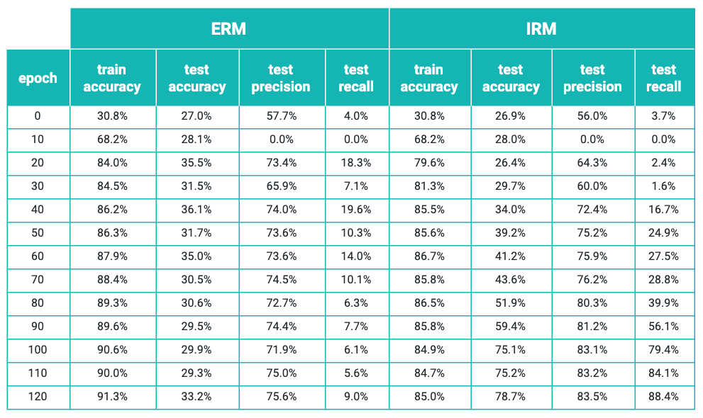
ERM outperforms the baseline in all environments, but not by too much in the new test environment. This can be attributed to the learning of spurious correlations. The network was able to effectively distinguish between raccoons and coyotes in the training environments, but the features it relied upon to do so were not general enough to help prediction much in the test environment.
In contrast, IRM loses a single percentage point of accuracy in the train environments, but performs almost as well in the test environment. The feature representation IRM constructs has translated between different environments effectively, and proves an effective discriminator.
As a practical point, we found that IRM worked best when the additional IRM penalty term was not added to the loss until the point at which ERM had reached its best performance - in this case the 40th training epoch. As such, ERM and IRM had identical training routines and performance until this point. When we introduced the IRM penalty, the IRM procedure continued to learn and gain out-of-distribution generalization capability, whereas ERM began to overfit. By the 120th epoch, IRM had the accuracy reported above, whereas ERM had achieved 91% in the combined training environments, at the cost of reducing its test accuracy by a few percentage points to 33%.
Interpretability
IRM yields impressive results, especially considering how hard it is to learn from these images. It has a clear and significant improvement in when compared to ERM in a new environment. In this section, we examine a few concrete examples of successes and failures of our prototype model and our speculations as to why they may be.
It would be nice to have a better sense of whether IRM has learned invariant features. By that we mean, whether it has learned to spot a raccoon’s long bushy tail or a coyote’s slender head, instead of the terrain or foliage in the image. Understanding which parts of the image contribute towards IRM’s performance is a powerful proposition. The classification task itself is hard: if you closely look at some of the images in the Wildcam dataset, at a first glance it’s even hard for us, humans, to point out where exactly the animal is. An interpretability technique like Local Interpretable Model-agnostic Explanations (LIME) provides valuable insights into how that classification is working.
LIME is an explanation technique that can be applied to almost any type of classification model — our report FF06: Interpretability discusses these possibilities — but here we will consider its application to image data. LIME is a way to understand how different parts of an input affect the output of a model. This is accomplished, essentially, by turning the dials of the input and observing the effect on the output.
Let’s first try and understand how LIME works at a high level - including what inputs we need to provide, and what to expect as output - through a sample image in the test set. The image on the left of the figure below is a sample raw image of a coyote with dimensions height=747 and width=1024, as were all images in the dataset.
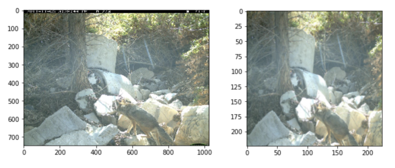
To use the IRM model, we must first perform some image transformations like resizing, cropping, and normalization - using the same transformations that we did when training the model. The input image then appears as shown on the right of the figure above, a normalized, 224 * 224 image. The transformed image when scored by the IRM model outputs a probability of 98% (0.98) for the coyote class! So yes, our model is pretty confident of its prediction.
Now, let’s see how LIME works on this image. First, LIME constructs a local linear model, and makes a prediction for the image. For the example image, the predicted score is 0.95, pretty close to the IRM model. When trying to explain the prediction, LIME uses interpretable representations. For images, interpretable representations are basically contiguous patches of similar pixels called superpixels. The superpixels for an image are generated by a standard algorithm, QuickShift, in the LIME implementation. The left panel in the figure below shows all of the 34 superpixels generated by LIME for the example image.
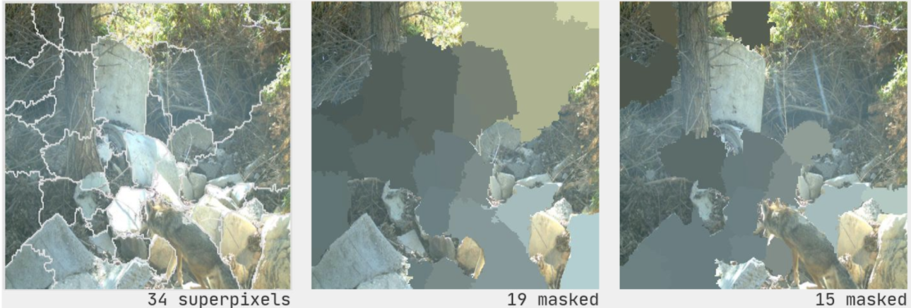
It then creates versions of the original image by randomly masking different combinations of the superpixels as shown in the middle and right panes of the above figure. Each random set of masked superpixels is one perturbation of the image. The modeler chooses the number of perturbations; in our case, we used 1000 perturbations of the original image. LIME then builds a regression model on all these perturbed images and determines the superpixels that contributed most towards the prediction, based on their weights.
The figure below shows the superpixel explanations (with the rest of the image grayed out) for the top 12 features that contribute towards the prediction of the coyote classification. While there are quite a few features that are mostly spurious covering the foliage or terrain, one of them covers the entire body of the coyote. Looking at these explanations provides an alternative way of assessing the IRM model and can enhance our trust that the model is learning to rely on sensible features.

Now when we generate the top 12 LIME explanations for the same image but based on the ERM model, they seem to capture more of the surroundings, rather than any of the coyote’s body parts.

And then there are instances where LIME explanations seem to rely on spurious features. For example, in the figure below, the original image is classified as a coyote by the IRM model with a probability of 72% (0.72), whereas the LIME score is close to 0.53. The superpixels contributing towards the classification for both the IRM and ERM models usually cover the terrain or foliage, though some outline the coyote’s body.

We observe that the explanations make more intuitive sense when the LIME score is close to the model score.
IRM can only learn to be invariant with respect to the invariants that the environments encode. If there are spurious correlations that are the same across environments, IRM will not distinguish them from invariant features.
One feature that appears invariant in this dataset is the day or night cycle. Raccoons appear exclusively at night, and IRM could well learn that night means raccoon, and rely on it heavily. This correlation is spurious; a raccoon is still a raccoon during the day! However, we would need more environments, including images of raccoons in the daytime, to disentangle that.
The representation that IRM extracts from an environment should theoretically be closer to encoding the latent causal structure of the problem than that which ERM extracts. In our scenario, we might expect that IRM learns to focus more on the actual animal in the picture, since the presence of the animal is the cause of a given annotation. The animals change little between environments, whereas environmental features (like foliage) are completely different at different camera trap locations. Thus, the causal features ought to be invariant between environments.
That said, although the IRM results appear promising for some samples, it is hard to confirm that there is an obvious pattern, and this can be attributed to both the model and the interpretability technique. We chose to train only the last layer of ResNet18 to come up with the IRM model. This choice has an inherent drawback: the capacity for feature learning is low. As such, we wouldn’t expect perfect results, since it’s unlikely that the pretrained ResNet representations map perfectly to raccoons and coyotes.[23]
Further, although an explanation of an image provides some reassurance of the quality of the model, it’s probably still insufficient to provide an overall picture of the kind of features a given model is using, aggregated from all the individual explanations. And even though explanations for multiple images are insightful, these have to be judiciously selected. When it comes to text or tabular data, there are ways to determine the global feature importances, because the features in tabular data or vocabulary stay consistent across all the data points. The superpixels of an image cannot be consistent across all the images, which makes it really hard to assess whether the explanations make sense. Developing tools to understand large image datasets is a worthy endeavour!
Product: Scene
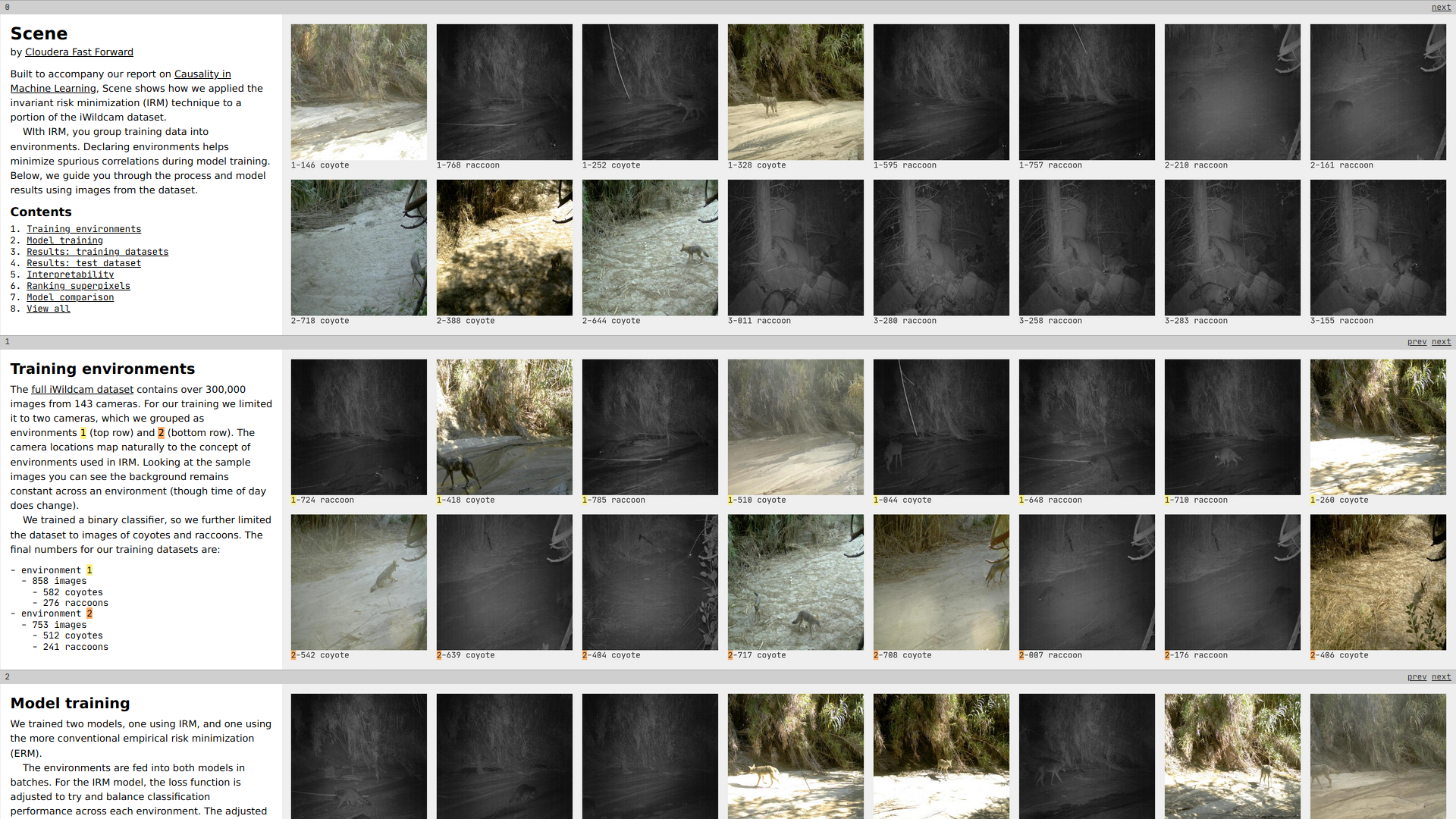
To accompany this report, we built a prototype called Scene that takes you on a guided tour through the dataset, models, and results of our experiment. With Scene, we really wanted to give people a feel for the images that make up the dataset. Each panel of the tour features 16 images from the dataset, cropped and resized to the same dimensions of the images that the model is trained on. Many of the images featured are randomly sampled from the dataset when we generate the page, while others we specifically selected to use as examples. We hope that the amount and variety of images shown helps people get an intuitive feel for the dataset.

If you want to go even deeper, we included an all page, which shows all 2,133 images in the dataset, along with the predictions and interpretability visualizations for each model. It’s nice to be able to use these visualizations to check intuitions (like which features are important to each model) with your own eyes. Of course, even having access to all the images doesn’t mean you can see “the big picture.” It’s difficult to hold everything you’ve seen in your head as you scroll through. If you’re not careful, you’ll end up generalizing the patterns you’ve seen most recently to the entire dataset. This is the challenge of visualizing the scale of the data that machine learning systems take in. Other techniques, like embeddings (as seen in our Active Learner prototype) can help you visualize patterns, but then you lose some of the detail gained by being able to see the images up close. No one technique can give you the whole picture; data visualization requires a variety of techniques.
Generating such a large number of images, complete with text labels and interpretability overlays, was an interesting technical challenge. Originally, we’d planned to have Scene animate transitions between the original image and the interpretability overlays. To do this efficiently in a browser, you generate a “sprite sheet” - a large image that contains all the different animation states you’ll transition through (a technique borrowed from video games). It was while we were generating the sprite sheets that we decided that, rather than transitioning through them one at a time, it would be more effective to show the entire sheet. Having more images visible together made comparisons easier and the scale of the dataset more clear. We ended up using the node-canvas package to crop and place the images, overlay the interpretability layers, and apply the labels through a node script. Since we do all the work of generating images locally, we guarantee the user as snappy an experience as possible. Static site generation has seen renewed interest as a web-development strategy, and could be especially useful for large-scale data-visualization.
Landscape
Causality spans a broad area of topics, including using causal insights to improve machine learning methods, adapting it for high-dimensional datasets and applying them for better data-driven decision making in real-world contexts. We also discussed in Causality and Invariance how the collected data is rarely an accurate reflection of the population, and hence may fail to generalize in different environments or new datasets. Methods based on invariance show promise in addressing out-of-distribution generalization.
Use Cases
As we demonstrated in the Prototype chapter, Invariant Risk Minimization is particularly well suited to image problems in diverse physical environments. However, an environment need not mean only the scenery in an image, and when it does, it need not be fixed to a single value. Here we suggest some applications in and beyond computer vision.
Healthcare
In healthcare, medical images have to be manually annotated by radiologists to identify abnormalities. These annotated images are then used to train and build diagnostic models. Often the devices (like MRI scanners) which generate these medical images exhibit some kind of variation.[24] That is, due to mechanical configurations, vendor differences, or any number of other reasons, the images that are generated by one MRI scanner could be systematically different from another for the same patient. As such, a diagnostic model that was built on the images generated by an old MRI scanner may perform poorly when tested on the images generated by a new scanner. One way to solve this problem is to have the radiologist annotate the images generated by the new scanner and then retrain the model. But that could be expensive and time-consuming. Plus, this isn’t a permanent solution; every time there’s a new scanner or changes to the configuration, it would be necessary to retrain the existing model with an entirely new set of images.
A diagnostic model based on invariant prediction that treats scanners as environments could be immune to these noisy device variations and change its decisions accordingly. This could save the time and money needed to annotate images from the new scanner.
Robotics
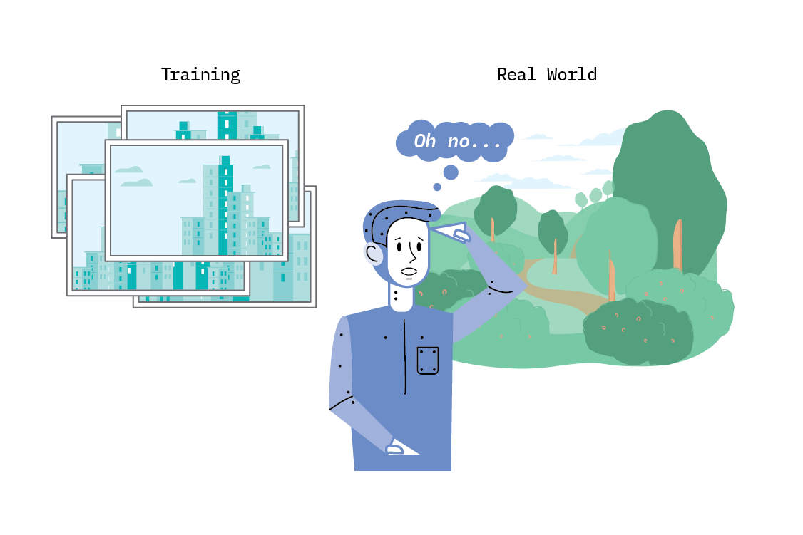
Autonomous systems need to detect and adapt to different environments. These systems rely on sophisticated sensors, cameras, and large amounts of labeled and diverse real-world datasets (which are difficult to acquire). Take, for example, the task of autonomously following a man-made trail that is traversed by hikers or mountain bikers. This is a mostly unsolved task for robotics, but yet an important one for applications like search and rescue.[25]
While many types of robots (such as the quadrupedal robot) can be efficient at locomotion, successfully navigating real-world forest trails is hard. Apart from the mechanics of the problem, perceiving real-world trails is difficult. The appearance of the wilderness area may vary a lot depending on the location, unpaved roads generally have less structure (and tend to blend in with the surrounding grass areas, vegetation, and such), and trails change over time. It would be impossible to have a comprehensive dataset of all trails, in all weather and lighting conditions.
In such cases, a possible solution is to cast the trail perception problem as an image classification task and adopt an invariance based approach that operates directly on the image’s raw pixel values. Successful application could allow for out-of-distribution generalization to new trails, since the features learned are more transferable than environment-specific signals. Naturally, similar ideas are relevant for autonomous vehicles in urban areas.
Activity recognition systems
Smart devices (phones, watches, fitness trackers) carry a large array of sensors: accelerometers, gyroscopes, magnetometers, barometers, ambient lights sensors, and many more. Categorizing this data by the activity being performed at the time of recording - such as sitting, standing, or swimming - has allowed for the development of machine learning-based human-activity recognition systems. Correctly predicting a wearer’s activity enables a host of contextual applications, in particular in (but not restricted to) the health and wellness space.[26]
Unfortunately, it is hard to satisfactorily model this data due to the diversity exhibited in the real world. A single individual can perform a given activity slightly differently day-to-day, or the device may be unusually placed, or held or worn in a variety of orientations. Of course, different users are also physically diverse, and devices have intrinsic differences in their sensors and systems. This means that we either need a labeled dataset that captures the activity for each user and device (which is prohibitively expensive) or another way of identifying attributes that generalize better. Methods based on invariance could be particularly useful and well-suited in this scenario, capturing the essence of “sitting,” rather than the particular sensor activations for a particular user sitting on a particular chair.
Natural language processing
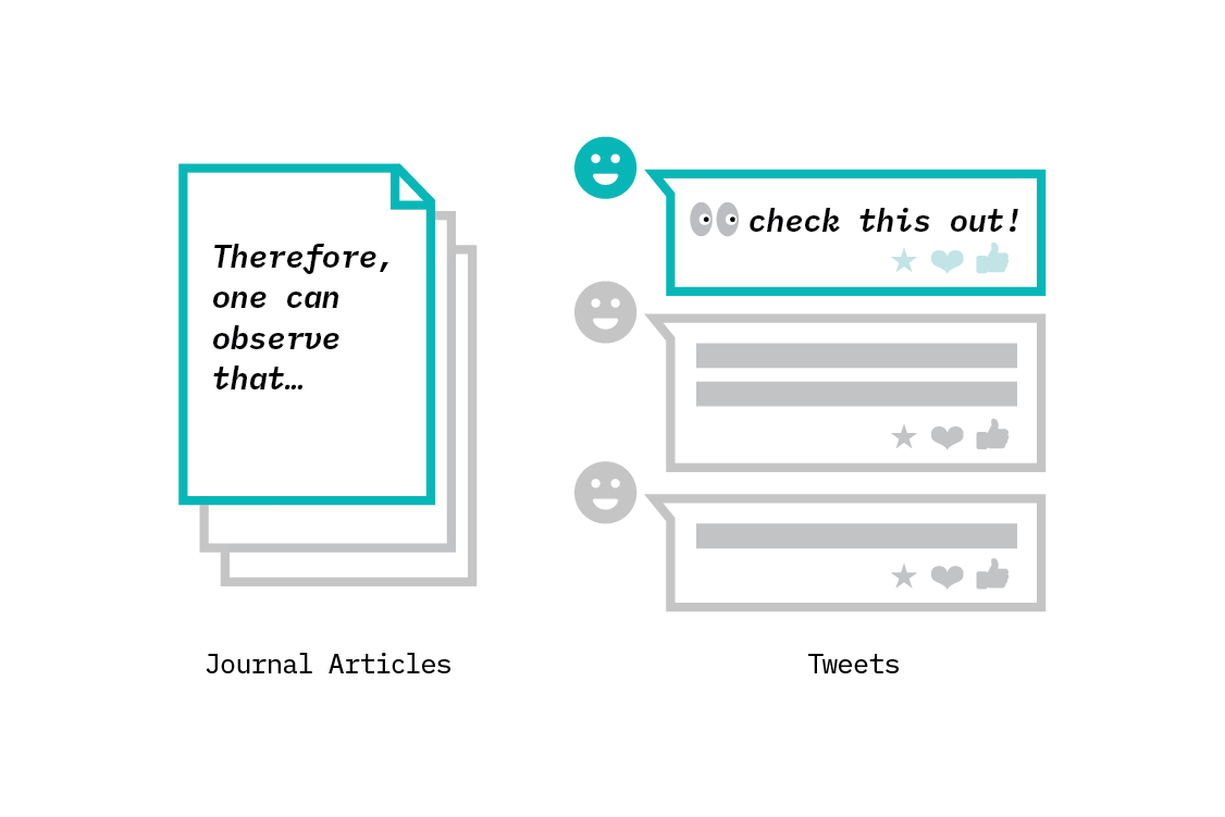
Invariant prediction approaches are of course not restricted exclusively to image problems. In natural language processing, texts from different publication platforms are tricky to analyze due to different contexts, vocabularies, and differences between how authors express themselves. For instance, financial news articles use a vocabulary and tone that differs from culture or society articles. The former is likely terse, whereas the latter may have an entertaining or personal tone. Similarly, online product reviews are linguistically different from tweets. Sentiment classification also relies heavily on context; different words are used to express whether someone likes a book versus an electronic gadget.
Two recent papers, An Empirical Study of Invariant Risk Minimization and Invariant Rationalization, apply the idea of IRM to a sentiment classification task, and find it improves out-of-distribution generalization. In particular, invariance acts to remove spurious reliance on single words which correlate highly with the target. Like images, text corpora form very high-dimensional datasets (there are many possible words!), making spurious correlations extremely unlikely to be noticed “manually.” As such, invariance based approaches are especially promising here.
Recommender systems
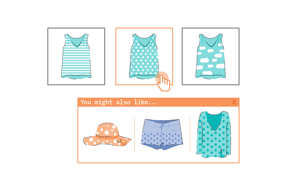
Recommendation systems are algorithms designed to present relevant items to users on the web (for example, suggesting which movie to watch, a book to read, or a product to buy). As such, making good recommendations is an important problem: we want to make relevant recommendations for a user based on a record of their historical activities, from which we must infer their preferences.
The training data is either explicit (e.g., a rating a user left on a book) or implicit (e.g., linger time on a webpage or click data). There is a well-known exposure problem in recommender systems: a user simply cannot click on an item with which they have not been presented. Modeling the data without accounting for this is akin to the assumption of independent and identically distributed data, and is false: users do not select items randomly and independently of one another. For instance, a user may choose between two competing movies to watch, rather than selecting whether to watch each independently.
RecSys are a classic application for causality, which allows us to correct for this exposure bias by treating the selection of items to present to a user as an intervention. Applying causal approaches to recommendation naturally improves generalization to new data,[27] and it seems likely that methods using invariant prediction could enhance this.
Tools
The invariance-based approaches to causality we have discussed do not require dedicated tooling - ICP and IRM are procedures that could be implemented with general purpose machine learning frameworks.
Nonetheless, the authors of the ICP papers [28] provide corresponding R packages: InvariantCausalPrediction and nonlinearICP. The packages make the techniques easy to use, and include additional utilities, such as dedicated plots for confidence intervals on causal coefficients. We are not aware of a package for IRM, but the authors have provided a code repository which reproduces the paper results.
Below, we list a handful of open source projects that aid in traditional, SCM-based causal inference.
DoWhy
Microsoft Research is developing the DoWhy python library for causal inference, incorporating elements of both causal graphical models and potential outcomes. The library is oriented around pandas DataFrames, and fits easily into a Python data analysis workflow. In particular, DoWhy makes a separation between four stages of causal inference:
- Modeling - defining a causal graph, or else the assumptions necessary for a potential outcomes approach (the common causes of the treatment and the outcome variable).
- Identification - identifying the expression it is necessary to evaluate, in terms of conditional probability distributions.
- Estimation - estimating the treatment effect. There are many estimation methods available in DoWhy, including machine learning-based methods from another of Microsoft’s causal libraries: EconML.
- Refutation - assessing the robustness of the conclusion. Given the reliance of causal inference on modeling assumptions, it is especially important to find ways to test our conclusions. DoWhy provides several methods for this, such as introducing a dummy common cause or replacing the treatment with a random placebo.
In addition to the above, DoWhy includes a novel algorithm, the “do-sampler.” In much of causal inference, the quantity of interest is a single number - for instance, the difference in the outcome variable when a binary treatment variable is applied (“what is the average causal effect of smoking on cancer incidence?”). The do-sampler extends the pandas DataFrame API directly, and moves beyond calculating causal effects to allow sampling from the full interventional distribution. Having done so, we can then compute arbitrary statistics under this intervention. The do-sampler is new, but provides a very promising direction for further research, and a potential avenue to making causal inference accessible to many more data science practitioners.
CausalDiscoveryToolbox
The Causal Discovery Toolbox provides implementations of many algorithms designed for causal discovery - attempting to recover the full causal graph from observational data alone. There are many approaches to causal discovery, and the library is relatively comprehensive, including algorithms for pairwise causal discovery (inferring the direction of causation between a pair of variables), graph skeleton creation (creating an undirected graph of potential causal relationships), and full graphical causal model discovery.
Discovery of entire causal graphs does not yet appear mature enough that we can naively trust its conclusions about the causal structure of a problem. This makes sense, given the difficulty of the task! Inferring the whole causal structure from only observational data is about the hardest imaginable problem we could face with data.
CausalNex
CausalNex is a very recently released (at time of writing) toolkit by QuantumBlack to help data scientists do causal reasoning. It provides both a graph structure learning component to help build the causal graph and tools to fit that graph as a Bayesian network.
The structure learning component is an implementation of DAGs with NOTEARS, an algorithm that casts structure learning as a continuous optimization problem. In its simplest form, it assumes linear relationships between variables (but unlike some causal discovery methods, does not assume Gaussian noise). Further, the algorithm assumes that all variables are observed (i.e., there is data for all variables). Unfortunately, this is rarely the case in causal problems.
Within these limitations, the algorithm is performant, and allows the user to specify hard constraints (such as, “these variables cannot be child nodes,” or “there is no causal relationship between these two variables”). This facilitates directly encoding domain knowledge into the graph, and using the structure learning component as an aid in places where the causal connection is not known.
Pyro
Uber’s Pyro probabilistic programming library is primarily intended for implementing deep probabilistic models and fitting them with variational inference. However, in addition to tools for conditioning on observed data, the library implements a do operation to force a variable to take a certain distribution. This allows simulating from interventional distributions, provided the structural causal model (including equations) is known. The intersection of probabilistic programming with causal inference is nascent, but promising!
Ethics
Machine learning is playing an increasingly critical role in our society. Decisions that were previously exclusively made by humans are more frequently being made algorithmically. These algorithmic systems govern everything from which emails reach our inboxes, to whether we are approved for credit, to whom we have the opportunity to date – and their impact on our experience of the world is growing. Furthermore, our understanding of how these systems work is still lacking. We can neither explain nor correct them when their predictions are unfairly discriminatory or their outputs are reinforcing existing biases. Causal reasoning gives us a framework for thinking about these problems.
Causal graphs make assumptions explicit
Even without employing the full machinery of causal inference, when one approaches a new problem, it can be informative to try to write down the causal graph. This forces us to confront our assumptions about a system. It also allows someone else to understand our assumptions, and furnishes a precise framework for debate.
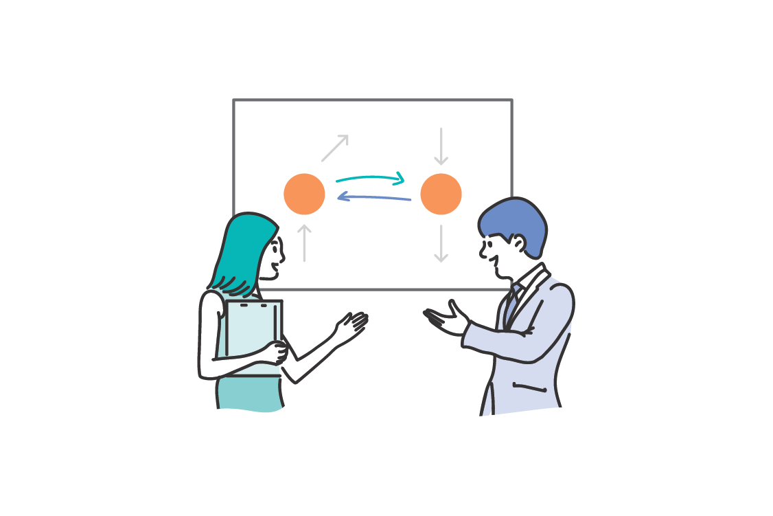
Making our assumptions explicit aids transparency, which is a win. However, it doesn’t protect against bad assumptions. Establishing causal relationships is hard. Unless we are able to perform sufficient experiments to validate our hypotheses, causal reasoning from observational data is subject to untested (sometimes untestable) assumptions.
We should make any causal claim with humility. As ever, we should be careful of dressing up a bad analysis with additional formalism.
Omitting protected attributes is not enough
It is unethical, and in many places illegal, to discriminate on the basis of a protected attribute, such as age, race, or disability. Avoiding direct discrimination (whereby some individuals with particular protected attributes are treated unfavourably) is comparatively easy. Appropriately, these protected attributes are frequently omitted from machine learning systems. Using a protected attribute as a feature directly is inviting discrimination based on that attribute.
More difficult to detect and avoid is indirect causal discrimination. Many features that are not themselves protected attributes are nonetheless highly predictive of a protected attribute. For instance, geographic location can correlate very highly with race, religion, and age. In denying loans to any individual with a particular zipcode, a bank could be committing indirect, but very real, discrimination against a protected attribute.
Another sub-category of discrimination is indirect spurious discrimination. These are instances when there are no pathways from causal attributes to the outcome. However, as we saw in From correlation to causation, correlations can arise from numerous causal structures. As such, merely omitting the protected attribute does not omit its effects. A system is not guaranteed to be non-discriminatory on a protected attribute simply because it does not include that attribute directly. More simply, just because a feature does not cause the target does not mean that it will not be predictive of the target. This presents a particular challenge to algorithmic systems that are designed to find subtle correlations, especially since much historical data on which algorithms are trained is subject to selection bias (and other biases).
Since removing protected attributes is not enough, we must evaluate the resulting model for its discrimination and fairness properties. There are many possible measures of fairness, and it is generally impossible to optimize for all of them.[29]
Several recent papers[30], for instance) have proposed causality as a route to understanding and defining fairness and discrimination. In particular, if we have a causal graphical model of a system, we can see which paths are impacted by protected attributes, and correctly account for that impact. There have also been contributions in non-parametric structural causal models that allow one to detect and distinguish the three main discriminations - namely, direct, indirect and spurious.[31]
That said, the difficulty lies in constructing the causal graph. A causal graph could, of course, be used to embed all kinds of biases and prejudices, but at least provides a basis for argument.
Invariance as a route to fairness
An interesting idea is proposed in the final section of the IRM paper: treating groups over which we want fairness as the environments. When we seek to learn an invariant model (be that by ICP or IRM), we are explicitly trying to learn a model that performs optimally in different environments. We could construct those environments by separating out groups having different values for protected attributes. Then, by learning a model that seeks to perform optimally in each environment, we are explicitly trying to guarantee the best performance for each protected attribute.
Said differently, invariant features are exactly those that are consistent across groups. Consider again a bank granting loans, this time directly to individuals. The bank does not wish to discriminate on the basis of protected attributes. By treating the protected attributes as the groups, they are looking to learn what impacts loan defaulting invariantly across those groups.
The idea of learning an invariant predictor across environments is that the representation used is capturing something true about the generative process of the data. This representation would be, to some degree, disentangled, in the sense that each dimension of the representation (a vector) should correspond to something meaningful. On the Fairness of Disentangled Representations shows experimentally that disentangled representations improve fairness in downstream uses.
Future
At the outset, causal reasoning provides a conceptual and technical framework for addressing questions about the effect of real or hypothetical actions or interventions. Once we understand what the effect of an action is, we can turn the question around and ask what action plausibly caused an event. This gives us a formal language to talk about cause-and-effect. That said, not every question about cause is easy to answer. Further, it may not be a trivial task to find an answer or even to interpret it. Causal graphs that we discuss in the Background: Causal Inference chapter provide a convenient way to discuss these notions, and allow us to reason about statistical dependencies in observed data.
Structural causal models take a step further to this intuitive way of reasoning by making formal assumptions about the parametric form of how the variables interact.
However, causal graphs and SCMs become difficult to construct as the number of variables increases. Some systems are hard to model in this way. How do we draw a causal graph for pixels of an image? Or words in text? The problem gets out of hand quickly.
Fortunately, not all problems require the entire causal graph. Often, we are interested only in the causal relations associated with one particular target variable. This is where methods based on invariance (like IRM) step in to allow the model to capture stable features across environments (that is, different data generating processes). This paradigm enables out-of-distribution generalization. As opposed to causal graphs or structural causal models, where the only way to validate assumptions of the variable interactions is through experimentation, IRM allows us to test them on an unseen test set!
Comparable approaches
So, at this point we probably agree that methods based on invariance are promising. How else might we approach out-of-distribution generalization? In general, there are two families of approaches; those that learn to match the feature distributions (or estimate a data representation) and those that employ some kind of optimization technique.
Domain adaptation
Domain adaptation is a special case of transfer learning. In domain adaptation, the model learns a task in a source domain, which has some feature distribution, and we would like it to be able to perform the same task well in a target domain, where the feature distribution is different. Domains play the same role as environments in invariance-based approaches; a source domain is an environment that was trained in, and a target domain is any environment that was not trained in.
Domain adaptation also enforces a kind of invariance - it seeks a representation that is distributed the same across source and target domains (so, across environments).[32] However, truly invariant, causal features need not follow the same distribution in different environments. A snowy cow will not generate quite the same pixel distribution as a sandy cow, and the causal feature we wish to represent is the cow itself.
Robust learning
The idea of learning across multiple environments is not novel to invariance-based approaches. Robust Supervised Learning is a family of techniques that uses the same multi-environment setup as IRM (but much predates it), with a similar goal of enabling or enhancing out-of-distribution generalization. Said differently, the goal is a predictor that is robust to distributional shifts of the inputs.
The difference from the IRM setup we have covered is the loss function. The key idea is to add environment-specific “baseline” terms to the loss, and try to fix these terms such that particularly noisy environments where the loss may be high do not dominate. Then, minimizing the loss should guarantee good performance across all the known environments. Further, a robust predictor will perform well in new environments that are interpolations of those seen in training. This certainly improves out-of-distribution generalization, but does not allow extrapolation outside of what was seen in training, whereas IRM can extrapolate, thanks to relying on an invariant predictor.
Meta-learning
Approaches like domain adaptation, robust learning, and (in general) transfer learning try to alleviate the problem of out-of-distribution generalization to some extent. Unfortunately, learning invariant features with varying distributions across environments is still challenging. These approaches are good at interpolation, but not extrapolation.
This is where meta-learning approaches like Model Agnostic Meta Learning (MAML)[33] come into play. The underlying idea for meta-learners generally is to attempt to learn tasks with a small number of labeled examples. Training meta-learners is a two-step process involving a learner and a trainer. The goal of the learner (model) is to quickly learn new tasks from a small amount of new data; hence, it is sometimes called a fast learner. (A task here refers to any supervised machine learning problem - e.g., predicting a class given a small number of examples.) This learner is trained, by the meta-learner, to be able to learn from a large number of different tasks. The meta-learner accomplishes this by repeatedly showing the learner hundreds and thousands of different tasks.
Learning then, happens at two levels. The first level focuses on quick acquisition of knowledge within each task with a few examples. The second level slowly pulls and digests information across all tasks. In case of MAML (which is optimization-based), the learner (or the first level) can achieve an optimal fast learning on a new task with only a small number of gradient steps because the meta-learner provides a good initialization of a model’s parameters. This approach is close to the problem of learning an optimal classifier in multiple environments, and could be explored further to learn invariant features within the data.
Some recent works have made the connection between causality and meta-learning explicitly.[34]
Looking ahead
In this section, we discuss future possibilities with causality in general, as well as with methods based on invariance.
Causal Reinforcement Learning
Reinforcement learning is the study of how an agent can learn to choose actions that maximize its future rewards in an interactive and uncertain environment. These agents rely on plenty of simulations (and sometimes real data) to learn which actions lead to high reward in a particular context. Causality is also about calculating the effect of actions, and allows us to transfer knowledge to new, unfamiliar situations. These two disciplines have evolved independently with little interaction between them until recently. Integrating them is likely to be a fruitful area of research, and may extend the reach of both causality and reinforcement learning.[35]
There is a natural mapping between the concept of intervention in causal inference and actions taken in reinforcement learning. Throughout an episode of reinforcement learning (an episode is formed of one run of the system, for example, a complete game of chess, or go), an agent takes actions. This defines a data generating process for the reward that the agent ultimately cares about; different sequences of actions will generate different rewards. Since the agent can choose its actions, each of them is an intervention in this data generating process. In making this connection, we can leverage the mathematics of causal inference. For instance, we could use counterfactuals, the third level of the The ladder of causation, to reason about actions not taken. Applying such causal techniques may reduce the state space the agent needs to consider, or help account for confounders.
Methods based on invariance, like IRM, in principle, learn to discover unknown invariances from multiple environments. We could leverage this attribute in reinforcement learning. An episode of RL consists of all the states that fall in between an initial state and a terminal state. Since each episode is independent of another, in IRM terminology they could be viewed as different environments. An agent could then learn robust policies from each of these episodes that leverage the invariant part of behaviour or actions that lead to reward.
While reinforcement learning itself is still in nascent stages when it comes to commercial applications, combining it with causality offers great potential.[36] But prior to that, we need to address some questions. For example, how do we combine programming abstractions in causal modeling with reinforcement learning to help find the best decisions? What tools and libraries are necessary to enable commercial applications in this space?
IRM and environments
IRM uses the idea of training in multiple environments to achieve out-of-distribution generalization. Unfortunately, few datasets come with existing environment annotations. There are at least two ways we can try to address this problem.
The first is to be mindful of the environment when collecting data, and collect metadata alongside it. This may be easy (for example, collecting the geo-location of photos in settings where this is possible and does not violate a user’s privacy), or extremely hard (requiring much post-collection manual labeling).
Another compelling but untested option is to try combining IRM with some sort of clustering to segment a single dataset into environments.[37] The question would be how to cluster in such a way that meaningful and diverse environments are defined. Since existing clustering approaches are purely correlative, and - as such - vulnerable to spurious correlations, this could prove challenging.
Studying the impact of environment selection, and how to create or curate datasets with multiple environments would be a valuable contribution to making invariance-based methods more widely applicable. (The authors of An Empirical Study of Invariant Risk Minimization reach the same conclusion.)
Causal reasoning for algorithmic fairness
In the Ethics chapter, we reviewed some notions of fairness in prediction problems and shared how tools of causal reasoning can be leveraged to address fairness. They depart in the traditional way of wholly relying on data-driven approaches and emphasize the need to require additional knowledge of the structure of the world, in the form of a causal model. This additional knowledge is particularly valuable, as it informs us how changes in variables propagate in a system (be it natural, engineered, or social). Explicit causal assumptions remove ambiguity from methods that just depend upon statistical correlations. Avoiding discrimination through causal reasoning is an active area of research. As efforts to aid more transparency and fairness in machine learning systems grow, causal reasoning will continue to gain significant momentum in guiding algorithms towards fairness.
Conclusion
Structural causal models give us a framework for thinking precisely about cause and effect, and encoding our assumptions about data generating processes. Knowing the complete model for a system is immensely powerful, allowing us to reason about how the system will behave when we intervene in the data generating process, and correct for selection biases.
In machine learning, we’re often concerned only with prediction, for which we do not need causal inference. However, even in this scenario, taking a causal approach brings some benefits. Notably, causal relationships are invariant (they do not change between environments) and when we learn predictors based on them, we get greatly improved out-of-distribution generalization.
For many problems, constructing a causal graph is prohibitively hard, and always relies on assumptions. When working with only observational data, these assumptions are especially important, since they cannot be validated through experiments. Fortunately, by relying on the correspondence between causal relationships and invariance, we can still construct the relevant part of the causal graph for some problems using Invariant Causal Prediction. For high dimensional inputs like image and text, we can use Invariant Risk Minimization to learn a predictor that greatly enhances our out-of-distribution performance by learning not to rely on dataset-specifc spurious correlations.
Research at the intersection of causality and machine learning is blossoming, with many major ML conferences hosting dedicated workshops on the topic. Invariance-based approaches are an especially promising development and are ripe for industrial application. As algorithmic systems become increasingly prevalent, and their influence on decisions grows, the need for causal reasoning becomes all the more acute. We think it is important that practitioners have an understanding of causality, and hope to see causal approaches gain significant traction in mainstream data science practice. We hope this report has sparked some causal curiosity in you!
See for instance, recent works by Yoshua Bengio, like A Meta-Transfer Objective for Learning to Disentangle Causal Mechanisms. ↩︎
See, for instance, Using Causal Inference to Improve the Uber User Experience. ↩︎
Facebook performed such an experiment in 2012, and received much criticism as a result. The ethical problem is not so much with the experiment itself, but rather that the subjects had not given informed consent, in violation of basic ethical guidelines for psychological research. ↩︎
An alternative popular framework is the Neyman-Reuben causal model, also known as Potential Outcomes. The frameworks are equivalent in that they can compute the same things, though some causal queries may be easier to reason about in one or the other. ↩︎
See also Pearl’s article: The Seven Tools of Causal Inference, with Reflections on Machine Learning. ↩︎
Some farm-experienced members of the CFF team are keen to point out that roosters crow pretty much all the time. ↩︎
On a technical note, correlation measures only linear association. For instance,
xsquared is uncorrelated withx, despite being completely dependent on it. When we say “correlation is not causation,” we really mean “statistical dependence is not causation.” ↩︎Alas, it requires a far more detailed technical knowledge than we can provide in this report. We recommend the textbook Causal Inference in Statistics: A Primer for a succinct introduction to Structural Causal Models. An abbreviated overview, (Causal Inference in Statistics: An Overview) is freely available as a PDF. The textbook Elements of Causal Inference (available through Open Access) also covers structural causal models, and includes several chapters explicitly drawing connections between causal inference and machine learning. ↩︎
We will examine the nuances of this statement in Causality and invariance. Correlation is predictive in distribution. ↩︎
Adam Kelleher and Amit Sharma have an excellent blog post describing this problem, and introducing a new causal sampling technology to make solving it easier. ↩︎
See Distinguishing cause from effect using observational data: methods and benchmarks. ↩︎
The scientific process of iterated hypothesis and experimentation can also be applied to constructing a causal model for business purposes. The popular George Edward Box quote is pertinent here: “all models are wrong, but some are useful” (see All models are wrong). ↩︎
Judea Pearl’s do-calculus is a set of rules to calculate exactly which variables we must account for - and how - to answer a given causal query in a potentially complicated graph. This is not trivial; often there are unobserved variables in a graph, and we must try to express the query only in terms of those variables for which we have data. ↩︎
There is a subtlety here. We said environments were defined by interventions. Naturally, it is impossible to intervene on the country a store is built in once the store is built. This turns out not to matter for the purposes of inferring the direct causal parents of the sales volume, so long as the country is further up the graph, and changing country alters the data generating process. ↩︎
Nonparametric conditional independence testing is an area of active research, and is generally hard - and made more so by having finite data. The nonlinear ICP paper also introduces the notion of defining sets; sometimes no single set of variables is accepted as the set of causal parents, but there are similar sets differing by only one or two variables that may be related. While the algorithm has failed to find a single consistent model, it is nonetheless conveying useful causal information. ↩︎
Longer than you may think! See, for instance, Machine perception of three-dimensional solids, published in 1963. ↩︎
The final section of the IRM paper includes a charming socratic dialogue that discusses this distinction, as well as the reason that regular supervised learning is so successful, from an invariance standpoint. ↩︎
See On Causal and Anticausal Learning for a description of the insight considering the causal direction of a problem brings to machine learning. ↩︎
Technically, loss is the error on the training set, and risk is the error across the whole data distribution. With finite training data, minimizing the loss on the training set is a proxy for minimizing the risk. ↩︎
Imperfect interpretability results notwithstanding, using ResNet as a feature extractor is representative of how CV systems are used in the real world, and the resulting out-of-distribution performance improvements are impressive. ↩︎
This example is given in An introduction to domain adaptation and transfer learning, and an empirical study using transfer learning was reported in Transfer Learning Improves Supervised Image Segmentation Across Imaging Protocols ↩︎
A Machine Learning Approach to Visual Perception of Forest Trails for Mobile Robots ↩︎
Scaling Human Activity Recognition via Deep Learning-based Domain Adaptation outlines the problem and some applications in this space. ↩︎
See Causal Inference for Recommendation and The Deconfounded Recommender: A Causal Inference Approach to Recommendation. ↩︎
Causal inference using invariant prediction: identification and confidence intervals and Invariant Causal Prediction for Nonlinear Models. ↩︎
See Inherent Trade-Offs in the Fair Determination of Risk Scores. ↩︎
See Causal Reasoning for Algorithmic Fairness and Avoiding Discrimination through Causal Reasoning. ↩︎
See Fairness in Decision-Making – The Causal Explanation Formula. ↩︎
Model-Agnostic Meta-Learning for Fast Adaptation of Deep Networks ↩︎
See A Meta-Transfer Objective for Learning to Disentangle Causal Mechanisms. ↩︎
There is a nice introduction to causal reinforcement learning in the paper Reinforcement learning and causal models. The blog post Introduction to Causal RL contains a shorter description, and also suggests some medical applications. ↩︎
We are grateful to David Lopez-Paz (one of the Invariant Risk Minimization authors) for sharing his thoughts and ideas about possible extensions and applications of IRM with us, including applications to reinforcement learning. ↩︎
This idea was also suggested to us by David Lopez-Paz. ↩︎